29 Track2KBA - Central Place Foragers: Clean and summarise data for analysis
Analyses outlined in this chapter were performed in R version 4.3.2 (2023-10-31 ucrt)
This chapter was last updated on 2024-02-23
29.1 What this chapter covers:
Suggested steps to cleaning data from central place foraging animals (e.g. seabirds during the breeding period that regularly return to nests)
Cleaning central place foraging data and preparing for the purpose of analysing the data using the Track2KBA R package
Deriving basic summary statistics about tracks of central place foraging animals
29.2 Outputs and assumptions of data within this chapter:
Two key outputs are derived:
A data frame of tracking data which has had tracks split into individual trips. The trip data has been cleaned via a speed filter and linear interpolation. Only complete trips are kept for further analyses.
A summary data frame of basic statistics about the tracking data
A key assumption:
- The use of complete trips only does not bias final outcomes.
29.3 Where you can get example data for the chapter:
This tutorial uses example data from a project led by the BirdLife International partner in Croatia: BIOM
The citation for this data is: Zec et al. 2023
Example data is available upon request
The example data: See chapter about merging tracking data
A description of the example data is given in a separate chapter
29.4 Load packages
Load required R packages for use with codes in this chapter:
If the package(s) fails to load, you will need to install the relevant package(s).
## ~~~~~~~~~~~~~~~~~~~~~~~~~~~~~~~~~~~~~~~~~~~~~~~~~~~~~~~~~~~~~~~~~~~~~~~~~~~~~
## Load libraries --------------------------------------------------------------
## ~~~~~~~~~~~~~~~~~~~~~~~~~~~~~~~~~~~~~~~~~~~~~~~~~~~~~~~~~~~~~~~~~~~~~~~~~~~~~

"Had to install R version: R version 4.2.2 (2022-10-31 ucrt) for aniMotum"
## [1] "Had to install R version: R version 4.2.2 (2022-10-31 ucrt) for aniMotum"## [1] "Animotum and CRAWL style interpolation in Appendix - not default comparison"## Options to install aniMotum package for animal track interpolation
## aniMotum: https://besjournals.onlinelibrary.wiley.com/doi/10.1111/2041-210X.14060
#install.packages('aniMotum', repos = c('https://ianjonsen.r-universe.dev', 'https://cloud.r-project.org'))
# may need to install aniMotum after downloading using: devtools::install_local(package.zip)
#install.packages('TMB', type = 'source')
#library("aniMotum")
## sf package for spatial data analyses (i.e. vector files such as points, lines, polygons)
library(sf)
## Tidyverse for data manipulation
library(tidyverse)
## ggplot2 for plotting opionts
library(ggplot2)
## rnaturalearth package for basemaps in R
library(rnaturalearth)
## leaflet package for interactive maps in R
#install.packages("leaflet")
library(leaflet)
##
library(purrr)
library(furrr)
#install.packages("track2KBA")
library(track2KBA)
## for date time
library(lubridate)
## for stats
library(stats)
## speed filter
library(trip)
## linear interpolation
library(adehabitatLT)29.5 Define object names for chapter
Typically, if your data follows the same format as the examples in the chapter (and previous chapters), then below should be the only thing(s) you need to change.
## ~~~~~~~~~~~~~~~~~~~~~~~~~~~~~~~~~~~~~~~~~~~~~~~~~~~~~~~~~~~~~~~~~~~~~~~~~~~~~
## Specify projections / store needed CRS definitions as variables ----
## SEE: https://epsg.io/
## ~~~~~~~~~~~~~~~~~~~~~~~~~~~~~~~~~~~~~~~~~~~~~~~~~~~~~~~~~~~~~~~~~~~~~~~~~~~~~

## world - unprojected coordinates
# wgs84 <- st_crs("EPSG:4326")


## ~~~~~~~~~~~~~~~~~~~~~~~~~~~~~~~~~~~~~~~~~~~~~~~~~~~~~~~~~~~~~~~~~~~~~~~~~~~~~
## Source a relevant basemap (download / or load your own)
## ~~~~~~~~~~~~~~~~~~~~~~~~~~~~~~~~~~~~~~~~~~~~~~~~~~~~~~~~~~~~~~~~~~~~~~~~~~~~~

## Source a world map from the rnaturalearth R package
## see details of function to change the type of map you get
## If you can't download this map - you may need to load a separate shapefile
## depicting a suitable basemap
# worldmap <- rnaturalearth::ne_download(scale = "large",
#                                        type = "countries",
#                                        category = "cultural",
#                                        destdir = tempdir(),
#                                        load = TRUE,
#                                        returnclass = "sf")
29.6 Load file (or file created from previous chapter)
## Read the csv file of merged tracking data that follows the output / download format
## of the Seabird Tracking Database
df_stdb_output <- read.csv("./data-testing/tracking-data/Puffinus-yelkouan-Z-tracking-STDB-output.csv")
NOTE: The example data used here is in the format of data downloaded from the Seabird Tracking Database. Your own data might not follow this format. However, many of the steps outlined below should be readily adaptable to your data so long as you modify column names or respective inputs accordingly.
29.7 dataGroup: prepare relevant grouping of data for analyses
See previous chapter which introduces the dataGroup concept - ensure your data is group accordingly when deriving a final output using the Track2KBA R package.
##                   dataset_id   scientific_name         common_name   site_name
## 1 populated-upon-upload-STDB Puffinus yelkouan Yelkouan Shearwater Lastovo SPA
## 2 populated-upon-upload-STDB Puffinus yelkouan Yelkouan Shearwater Lastovo SPA
##   colony_name lat_colony lon_colony device         bird_id        track_id
## 1           Z  42.774893  16.875649    GPS 19_Tag17600_Z-9 19_Tag17600_Z-9
## 2           Z  42.774893  16.875649    GPS 19_Tag17600_Z-9 19_Tag17600_Z-9
##            original_track_id   age     sex   breed_stage
## 1 populated-upon-upload-STDB adult unknown chick-rearing
## 2 populated-upon-upload-STDB adult unknown chick-rearing
##                 breed_status   date_gmt time_gmt  latitude longitude
## 1 populated-upon-upload-STDB 2019-05-24 00:49:09 42.811528 16.885531
## 2 populated-upon-upload-STDB 2019-05-24 01:09:03 42.812029 16.886907
##   argos_quality equinox
## 1            NA      NA
## 2            NA      NA
## Review the main columns of data separately. This helps check for errors associated
## with data entry. E.g. perhaps you typed chick-rearing and CHICK-rearing. Because
## of the difference in lower-case vs. upper-case text, you might accidentally consider
## these as separate components of your dataset.
## the table function is useful to check the unique number of entries per unique input
table(df_stdb_output$scientific_name)##
## Puffinus yelkouan
## 11354##
## Lastovo SPA
## 11354##
## Z
## 11354##
## populated-upon-upload-STDB
## 11354##
## chick-rearing
## 11354##
## adult
## 11354##
## unknown
## 11354## Summarise the data by species, site_name, colony_name, year, breed_status (if you have this), breed_stage, age, sex.
## First we add a new year column by splitting the date column so we can get information about years
df_overview <- df_stdb_output %>% mutate(year = year(date_gmt)) %>%
## then we group the data by relevant columns
group_by(scientific_name,
site_name,
colony_name,
year,
#breed_status, # if you downloaded data from the STDB, you should have this info.
breed_stage,
age,
sex,
device) %>%
## then we continue to summarise by the distinct number of entries per group
summarise(n_birds = n_distinct(bird_id),
n_tracks = n_distinct(track_id))
## review the summary output
df_overview## # A tibble: 2 × 10
## # Groups: scientific_name, site_name, colony_name, year,
## # breed_stage, age, sex [2]
## scientific_name site_name colony_name year breed_stage age sex device
## <chr> <chr> <chr> <dbl> <chr> <chr> <chr> <chr>
## 1 Puffinus yelkouan Lastovo SPA Z 2019 chick-rear… adult unkn… GPS
## 2 Puffinus yelkouan Lastovo SPA Z 2020 chick-rear… adult unkn… GPS
## # ℹ 2 more variables: n_birds <int>, n_tracks <int>29.7.1 dataGroup: Defining the dataGroup for the tutorial
From the summary above, we can see that we have data for:
One species
One colony
adult birds only
tracks from the chick-rearing period only
all tracked with GPS devices
tracked for two seasons
[From preliminary data exploration, we decided to pool tracks from the two years given birds were utilising the same areas]
[Insert Martin’s new paper about sample size / years of tracking data]
dataGroup for the tutorial is therefore defined as: Adult Puffinus yelkouan, tracked from colony Z, during the chick-rearing period.
- See the separate chapter about defining your dataGroup for analyses for further details.
29.8 dataGroup inspection: visual review
Here, we visually inspect the overall data to double check it generally looks correct.
A reminder on initial pre-filtering which may need to happen:
What should you look for when visualising the raw data? * Are your locations in realistic places? * Have you perhaps mixed up the latitude and longitude columns? * Does your data cross the international date line? Do you know how to deal with this? * Will you need to remove sections of the data that do not represent a time when the animal was tagged? (e.g. perhaps you set the device to start recording locations before deploying on the animal. So the tag might have recorded while you were travelling to the deployment location. Therefore, removing these sections of the track will facilitate your overall analysis.)
## quick plot of all data for a quick overview
dataGroup.plot <- st_as_sf(df_stdb_output, coords = c("longitude", "latitude"), crs=4326) # 4326 = geographic WGS84
plot(st_geometry(dataGroup.plot),
     cex = 0.5,
     pch = 1)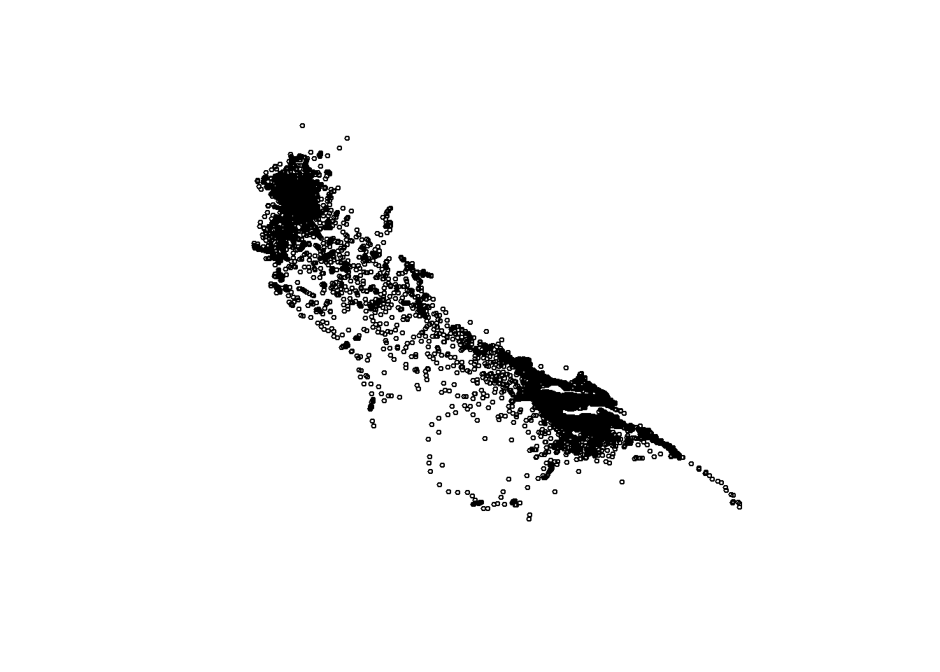
## [1] 11354## interactive plot
leaflet() %>% ## start leaflet plot
addProviderTiles(providers$Esri.WorldImagery, group = "World Imagery") %>%
## plot the points. Note: leaflet automatically finds lon / lat colonies
## Colour accordingly.
addCircleMarkers(data = df_stdb_output,
radius = 3,
fillColor = "cyan",
fillOpacity = 0.5, stroke = F) 29.9 Arrange data and remove duplicate entries
Once you have formatted your data into a standardised format and ensured that parts of your data is inputted correctly, it is also worth ensuring your data is ordered (arranged) correctly chronologically. An artifact of manipulating spatial data is that sometimes the data can become un-ordered with respect to time, or, given the way various devices interact with satellites, you can also end up with duplicated entries according to timestamps.
This can be a first problem, causing your track to represent unrealistic movement patterns of the animal.
We need to ensure our data is ordered correctly and also remove any duplicate timestamps.
##                   dataset_id   scientific_name         common_name   site_name
## 1 populated-upon-upload-STDB Puffinus yelkouan Yelkouan Shearwater Lastovo SPA
## 2 populated-upon-upload-STDB Puffinus yelkouan Yelkouan Shearwater Lastovo SPA
##   colony_name lat_colony lon_colony device         bird_id        track_id
## 1           Z  42.774893  16.875649    GPS 19_Tag17600_Z-9 19_Tag17600_Z-9
## 2           Z  42.774893  16.875649    GPS 19_Tag17600_Z-9 19_Tag17600_Z-9
##            original_track_id   age     sex   breed_stage
## 1 populated-upon-upload-STDB adult unknown chick-rearing
## 2 populated-upon-upload-STDB adult unknown chick-rearing
##                 breed_status   date_gmt time_gmt  latitude longitude
## 1 populated-upon-upload-STDB 2019-05-24 00:49:09 42.811528 16.885531
## 2 populated-upon-upload-STDB 2019-05-24 01:09:03 42.812029 16.886907
##   argos_quality equinox
## 1            NA      NA
## 2 NA NA## 'data.frame': 11354 obs. of 21 variables:
## $ dataset_id : chr "populated-upon-upload-STDB" "populated-upon-upload-STDB" "populated-upon-upload-STDB" "populated-upon-upload-STDB" ...
## $ scientific_name : chr "Puffinus yelkouan" "Puffinus yelkouan" "Puffinus yelkouan" "Puffinus yelkouan" ...
## $ common_name : chr "Yelkouan Shearwater" "Yelkouan Shearwater" "Yelkouan Shearwater" "Yelkouan Shearwater" ...
## $ site_name : chr "Lastovo SPA" "Lastovo SPA" "Lastovo SPA" "Lastovo SPA" ...
## $ colony_name : chr "Z" "Z" "Z" "Z" ...
## $ lat_colony : num 42.8 42.8 42.8 42.8 42.8 ...
## $ lon_colony : num 16.9 16.9 16.9 16.9 16.9 ...
## $ device : chr "GPS" "GPS" "GPS" "GPS" ...
## $ bird_id : chr "19_Tag17600_Z-9" "19_Tag17600_Z-9" "19_Tag17600_Z-9" "19_Tag17600_Z-9" ...
## $ track_id : chr "19_Tag17600_Z-9" "19_Tag17600_Z-9" "19_Tag17600_Z-9" "19_Tag17600_Z-9" ...
## $ original_track_id: chr "populated-upon-upload-STDB" "populated-upon-upload-STDB" "populated-upon-upload-STDB" "populated-upon-upload-STDB" ...
## $ age : chr "adult" "adult" "adult" "adult" ...
## $ sex : chr "unknown" "unknown" "unknown" "unknown" ...
## $ breed_stage : chr "chick-rearing" "chick-rearing" "chick-rearing" "chick-rearing" ...
## $ breed_status : chr "populated-upon-upload-STDB" "populated-upon-upload-STDB" "populated-upon-upload-STDB" "populated-upon-upload-STDB" ...
## $ date_gmt : chr "2019-05-24" "2019-05-24" "2019-05-24" "2019-05-24" ...
## $ time_gmt : chr "00:49:09" "01:09:03" "01:29:03" "01:49:09" ...
## $ latitude : num 42.8 42.8 42.8 42.8 42.8 ...
## $ longitude : num 16.9 16.9 16.9 16.9 16.9 ...
## $ argos_quality : logi NA NA NA NA NA NA ...
## $ equinox : logi NA NA NA NA NA NA ...## NULL## merge the date and time columns
df_stdb_output$dttm <- with(df_stdb_output, ymd(date_gmt) + hms(time_gmt))
## first check how many duplicate entries you may have. If there are many, it
## is worth exploring your data further to understand why.
n_duplicates <- df_stdb_output %>%
group_by(bird_id, track_id) %>%
arrange(dttm) %>%
dplyr::filter(duplicated(dttm) == T)
## review how many duplicate entries you may have. Print the message:
print(paste("you have ",nrow(n_duplicates), " duplicate records in a dataset of ",
nrow(df_stdb_output), " records.", sep =""))## [1] "you have 11 duplicate records in a dataset of 11354 records."## remove duplicates entries if no further exploration is deemed necessary
df_stdb_output <- df_stdb_output %>%
## first group data by individual animals and unique track_ids
group_by(bird_id, track_id) %>%
## then arrange by timestamp
arrange(dttm) %>%
## then if a timestamp is duplicated (TRUE), then don't select this data entry.
## only select entries where timestamps are not duplicated (i.e. FALSE)
dplyr::filter(duplicated(dttm) == F)29.10 Speed filter GPS data: remove erroneous location points
It’s often the case that some location points will be in artificial places (i.e. the wrong places). This can happen for many reasons.
To automatically remove some of these artifical locaiton points prior to analyses, one can apply a speed filter.
Here we use the McConnel Speed Filter.
##                   dataset_id   scientific_name         common_name   site_name
## 1 populated-upon-upload-STDB Puffinus yelkouan Yelkouan Shearwater Lastovo SPA
## 2 populated-upon-upload-STDB Puffinus yelkouan Yelkouan Shearwater Lastovo SPA
##   colony_name lat_colony lon_colony device         bird_id        track_id
## 1           Z  42.774893  16.875649    GPS 19_Tag17652_Z-2 19_Tag17652_Z-2
## 2           Z  42.774893  16.875649    GPS 19_Tag17652_Z-2 19_Tag17652_Z-2
##            original_track_id   age     sex   breed_stage
## 1 populated-upon-upload-STDB adult unknown chick-rearing
## 2 populated-upon-upload-STDB adult unknown chick-rearing
##                 breed_status   date_gmt time_gmt  latitude longitude
## 1 populated-upon-upload-STDB 2019-05-01 21:40:41 42.815077 16.890582
## 2 populated-upon-upload-STDB 2019-05-01 22:00:41 42.837505 16.897495
##   argos_quality equinox                dttm
## 1            NA      NA 2019-05-01 21:40:41
## 2            NA      NA 2019-05-01 22:00:41
## [1] 34## Define maximum speed in km/h (kilometers per hour)
speed.filter.threshold <- 100 ## Important number to change depending on whether you have flying or non-flying seabirds
## create blank data frame to capture filtered tracks and summary data
tracks_speed <- data.frame()
tracks_speed_summary <- data.frame()
##
for(i in 1:length(unique(df_stdb_output$bird_id))){
temp <- df_stdb_output %>% dplyr::filter(bird_id == unique(df_stdb_output$bird_id)[i])
## remove any erroneous locations due to speed use the McConnel Speed Filter
##from the trip package
trip_obj <- temp %>%
group_by(bird_id) %>%
dplyr::select(x = latitude,
y = longitude,
dttm,
everything()) %>%
trip()
## McConnel Speedilter -----
## apply speedfilter and create data frame
trip_obj$Filter <- speedfilter(trip_obj, max.speed = speed.filter.threshold) # speed in km/h
trip_obj <- data.frame(trip_obj)
#head(trip_obj,2)
#dim(trip_obj)
## Keep only filtered coordinates - after checking dimensions of other outputs again
trip_obj <- subset(trip_obj,trip_obj$Filter==TRUE)
## bind back onto dataframe
tracks_speed <- rbind(tracks_speed, trip_obj)
## Populate summary data
temp_summary <- data.frame(bird_id = temp$bird_id[1],
n_points_PreFilter = nrow(temp),
n_points_PostFilter = nrow(trip_obj),
points_removed = ifelse(nrow(temp)-nrow(trip_obj) > 0, "Yes", "No"))
## bind on summary information
tracks_speed_summary <- rbind(tracks_speed_summary, temp_summary)
## remove temporary items before next loop iteration
rm(temp,trip_obj, temp_summary)
## Print loop progress
print(paste("Track ", i, " of ", length(unique(df_stdb_output$bird_id)), " processed"))
}## [1] "Track 1 of 34 processed"
## [1] "Track 2 of 34 processed"
## [1] "Track 3 of 34 processed"
## [1] "Track 4 of 34 processed"
## [1] "Track 5 of 34 processed"
## [1] "Track 6 of 34 processed"
## [1] "Track 7 of 34 processed"
## [1] "Track 8 of 34 processed"
## [1] "Track 9 of 34 processed"
## [1] "Track 10 of 34 processed"
## [1] "Track 11 of 34 processed"
## [1] "Track 12 of 34 processed"
## [1] "Track 13 of 34 processed"
## [1] "Track 14 of 34 processed"
## [1] "Track 15 of 34 processed"
## [1] "Track 16 of 34 processed"
## [1] "Track 17 of 34 processed"
## [1] "Track 18 of 34 processed"
## [1] "Track 19 of 34 processed"
## [1] "Track 20 of 34 processed"
## [1] "Track 21 of 34 processed"
## [1] "Track 22 of 34 processed"
## [1] "Track 23 of 34 processed"
## [1] "Track 24 of 34 processed"
## [1] "Track 25 of 34 processed"
## [1] "Track 26 of 34 processed"
## [1] "Track 27 of 34 processed"
## [1] "Track 28 of 34 processed"
## [1] "Track 29 of 34 processed"
## [1] "Track 30 of 34 processed"
## [1] "Track 31 of 34 processed"
## [1] "Track 32 of 34 processed"
## [1] "Track 33 of 34 processed"
## [1] "Track 34 of 34 processed"## x y dttm dataset_id
## 1 42.815077 16.890582 2019-05-01 21:40:41 populated-upon-upload-STDB
## 2 42.837505 16.897495 2019-05-01 22:00:41 populated-upon-upload-STDB
## scientific_name common_name site_name colony_name lat_colony
## 1 Puffinus yelkouan Yelkouan Shearwater Lastovo SPA Z 42.774893
## 2 Puffinus yelkouan Yelkouan Shearwater Lastovo SPA Z 42.774893
## lon_colony device bird_id track_id original_track_id
## 1 16.875649 GPS 19_Tag17652_Z-2 19_Tag17652_Z-2 populated-upon-upload-STDB
## 2 16.875649 GPS 19_Tag17652_Z-2 19_Tag17652_Z-2 populated-upon-upload-STDB
## age sex breed_stage breed_status date_gmt time_gmt
## 1 adult unknown chick-rearing populated-upon-upload-STDB 2019-05-01 21:40:41
## 2 adult unknown chick-rearing populated-upon-upload-STDB 2019-05-01 22:00:41
## argos_quality equinox Filter optional
## 1 NA NA TRUE TRUE
## 2 NA NA TRUE TRUE## bird_id n_points_PreFilter n_points_PostFilter
## 1 19_Tag17652_Z-2 498 498
## 2 19_Tag40073_Z-1 641 641
## 3 19_Tag17617_Z-4 (2nd Parent) 177 177
## 4 19_Tag40069_Z-6 287 287
## 5 19_Tag40170_Z-12 418 418
## 6 19_Tag40078_Z-3 (2nd Parent) 65 65
## 7 19_Tag17704_Z-11 227 226
## 8 19_Tag17604_Z-7 152 152
## 9 19_Tag40133_Z-15 133 133
## 10 19_Tag40118_Z-2 (2nd Parent) 373 373
## 11 19_Tag40066_Z-14 209 209
## 12 19_Tag40182_Z-4 308 308
## 13 19_Tag17735_Z-3 (RAW DATA MISSING) 502 502
## 14 19_Tag40138_Z-17 337 337
## 15 19_Tag17600_Z-9 310 310
## 16 19_Tag40094_Z-16 228 228
## 17 19_Tag40177_Z-17 (2nd Parent) 596 596
## 18 19_Tag40086_Z-11 (2nd Parent) 351 351
## 19 19_Tag17644_Z-13 243 243
## 20 20_Tag40193_Z-13 (2nd Parent) 65 65
## 21 20_Tag41108_Z-95 (2nd Parent) 502 502
## 22 20_Tag17604_Z-95 274 274
## 23 20_Tag17600_Z-170 267 267
## 24 20_Tag40094_Z-131 462 462
## 25 20_Tag40073_Z-131 (2nd Parent) 469 469
## 26 20_Tag40133_Z-1 (2nd Parent) 641 641
## 27 20_Tag40118_Z-175 746 745
## 28 20_Tag17677_Z-170 (2nd Parent) 147 147
## 29 20_Tag40078_Z-178 270 270
## 30 20_Tag17724_Z-106 (2nd Parent) 4 4
## 31 20_Tag40024_Z-178 (2nd Parent) 490 490
## 32 20_Tag40039_Z-15 (2nd Parent) 571 571
## 33 20_Tag17644_Z-106 345 345
## 34 20_Tag40859_Z-179 35 35
## points_removed
## 1 No
## 2 No
## 3 No
## 4 No
## 5 No
## 6 No
## 7 Yes
## 8 No
## 9 No
## 10 No
## 11 No
## 12 No
## 13 No
## 14 No
## 15 No
## 16 No
## 17 No
## 18 No
## 19 No
## 20 No
## 21 No
## 22 No
## 23 No
## 24 No
## 25 No
## 26 No
## 27 Yes
## 28 No
## 29 No
## 30 No
## 31 No
## 32 No
## 33 No
## 34 No## update column names in speed filtered tracks
tracks_speed <- tracks_speed %>%
mutate(latitude = x,
longitude = y)29.11 Speed filter PTT data: remove erroneous location points
Examples to be added to appendix showcasing how to speed filter PTT data.
29.12 Speed filter data review: plotting
Plot the track of an animal with speed filtered data versus non-filtered data.
Note: plotting with the leaflet package in RStudio requires an internet connection.
## Get the ID of the first example track of animal with speed filtered data
example_animal <- tracks_speed_summary %>%
  dplyr::filter(points_removed == "Yes") %>%
  slice(1) %>%
  dplyr::select(bird_id)

## Get the original data
non.speed.filtered <- df_stdb_output %>% dplyr::filter(bird_id == example_animal$bird_id)

## Get the speed filtered ata
speed.filtered <- tracks_speed %>% dplyr::filter(bird_id == example_animal$bird_id)

## plot original vs speedfiltered data

## interactive plot
leaflet() %>% ## start leaflet plot
  addProviderTiles(providers$Esri.WorldImagery, group = "World Imagery") %>%
  ## plot the points. Note: leaflet automatically finds lon / lat colonies
  ## Colour accordingly.
  ## ORIGINAL TRACK
  addCircleMarkers(data = non.speed.filtered,
                   radius = 3,
                   fillColor = "red",
                   fillOpacity = 1,
                   stroke = F) %>%
  ## Plot lines between original track points
  addPolylines(lng = non.speed.filtered$longitude,
               lat = non.speed.filtered$latitude, weight = 1,
               color = "red") %>%
  ## SPEED FILTERED TRACK
  addCircleMarkers(data = speed.filtered,
                   #label = bird_track$nlocs,
                   radius = 3,
                   fillColor = "cyan",
                   fillOpacity = 1,
                   stroke = F) %>%
## plot lines between speed filtered points
  addPolylines(lng = speed.filtered$longitude,
               lat = speed.filtered$latitude, weight = 1,
               color = "cyan")
29.13 Data cleaning for CPF: n_locs, sampling interval, interpolation
So far, the following data cleaning steps have been applied:
General review of spatial data
Removing - if necessary - sections of tracks when animals were not tracked but devices were recording information (example code / procedures to be provided in future versions of toolkit)
Arranging data chronologically and removing duplicate entries
Speed filter for clearly erroneous location points
Further cleaning of data will typically be necessary for many analyses. Steps may include:
Removing data with too few location points
Reviewing the sampling frequency of data (i.e. what frequncy you set your devices to record at versus what they actually recorded at)
Interpolating data to generate tracking information that approximates an even sampling interval
When to clean data with respect to the steps above may depend on the type of animal you tracked.
29.13.1 Data cleaning for CPF seabirds: tracks vs. trips
If you have been tracking central place foraging animals, especially with modern tracking devices, it’s likely that you will have many trips recorded from an individual that was tracked.
Defining trips: For the purpose of analysing central place foraging data with track2kba, we consider a unique trip to be the period of time from when an animal departs its colony (or particular nest), to the moment it returns to the colony (or particular nest).
Therefore, if we have tracking information from individuals over sufficient time period, it’s likely you will have recorded information about multiple trips.
We need to split the information into unique trips.
Functions in the track2kba R package can help us do this.
29.13.2 Data cleaning for CPF seabirds: Nesting habitat considerations
For CPF species that nest in burrows, forests, or other locations where satellite signals may become interrupted for extend periods of time, it can be worth first splitting the overall tracking information into individual trips before filtering or cleaning data further according to number of locations (n_locs) or recorded sampling frequency.
EXAMPLE DATA CONSIDERATIONS (Burrow nesting species): Puffinus yelkouan is a burrow nesting species. Therefore, we expect to have long gaps in the tracking information while the birds are sitting on nests (because satellite signals with the tracking device will be interuppted). For this reason, we will first split the tracking information into individual trips, and then apply further filters. Otherwise, it may appear that there are artificially large gaps in your tracking data.
If you have tracking information from a species where satellite signal is unlikely to be interuppted from permanent features such as burrows or trees, it may be suitable to filter your data further before splitting tracks into individual trips because data is unlikely to be as biased by the presence of permanent physical features.
29.14 track2KBA: format data for use
29.14.1 track2KBA::formatFields()
This function will help format your data to align with that required of track2KBA.
In other words: for the track2KBA functions to work, your data needs to have certain columns named in the appropriate way. This function will help with that.
We apply the formatting to the most recently filtered data.
## Format the key data fields to the standard used in track2KBA
dataGroup <- formatFields(
  ## your input data.frame or tibble
  dataGroup = tracks_speed,
  ## ID of the animal you tracked
  fieldID   = "bird_id",
  ## date in GMT
  fieldDate = "date_gmt",
  ## time in GMT
  fieldTime = "time_gmt",
  ## longitude of device
  fieldLon  = "longitude",
  ## latitude of device
  fieldLat  = "latitude"
)

## Check output. Output is a data.frame
head(dataGroup,2)
## x y dttm dataset_id
## 1 42.815077 16.890582 2019-05-01 21:40:41 populated-upon-upload-STDB
## 2 42.837505 16.897495 2019-05-01 22:00:41 populated-upon-upload-STDB
## scientific_name common_name site_name colony_name lat_colony
## 1 Puffinus yelkouan Yelkouan Shearwater Lastovo SPA Z 42.774893
## 2 Puffinus yelkouan Yelkouan Shearwater Lastovo SPA Z 42.774893
## lon_colony device ID track_id original_track_id
## 1 16.875649 GPS 19_Tag17652_Z-2 19_Tag17652_Z-2 populated-upon-upload-STDB
## 2 16.875649 GPS 19_Tag17652_Z-2 19_Tag17652_Z-2 populated-upon-upload-STDB
## age sex breed_stage breed_status date_gmt time_gmt
## 1 adult unknown chick-rearing populated-upon-upload-STDB 2019-05-01 21:40:41
## 2 adult unknown chick-rearing populated-upon-upload-STDB 2019-05-01 22:00:41
## argos_quality equinox Filter optional Latitude Longitude DateTime
## 1 NA NA TRUE TRUE 42.815077 16.890582 2019-05-01 21:40:41
## 2 NA NA TRUE TRUE 42.837505 16.897495 2019-05-01 22:00:41## 'data.frame': 11341 obs. of 27 variables:
## $ x : num 42.8 42.8 42.8 42.8 42.8 ...
## $ y : num 16.9 16.9 16.9 16.9 16.9 ...
## $ dttm : POSIXct, format: "2019-05-01 21:40:41" "2019-05-01 22:00:41" ...
## $ dataset_id : chr "populated-upon-upload-STDB" "populated-upon-upload-STDB" "populated-upon-upload-STDB" "populated-upon-upload-STDB" ...
## $ scientific_name : chr "Puffinus yelkouan" "Puffinus yelkouan" "Puffinus yelkouan" "Puffinus yelkouan" ...
## $ common_name : chr "Yelkouan Shearwater" "Yelkouan Shearwater" "Yelkouan Shearwater" "Yelkouan Shearwater" ...
## $ site_name : chr "Lastovo SPA" "Lastovo SPA" "Lastovo SPA" "Lastovo SPA" ...
## $ colony_name : chr "Z" "Z" "Z" "Z" ...
## $ lat_colony : num 42.8 42.8 42.8 42.8 42.8 ...
## $ lon_colony : num 16.9 16.9 16.9 16.9 16.9 ...
## $ device : chr "GPS" "GPS" "GPS" "GPS" ...
## $ ID : chr "19_Tag17652_Z-2" "19_Tag17652_Z-2" "19_Tag17652_Z-2" "19_Tag17652_Z-2" ...
## $ track_id : chr "19_Tag17652_Z-2" "19_Tag17652_Z-2" "19_Tag17652_Z-2" "19_Tag17652_Z-2" ...
## $ original_track_id: chr "populated-upon-upload-STDB" "populated-upon-upload-STDB" "populated-upon-upload-STDB" "populated-upon-upload-STDB" ...
## $ age : chr "adult" "adult" "adult" "adult" ...
## $ sex : chr "unknown" "unknown" "unknown" "unknown" ...
## $ breed_stage : chr "chick-rearing" "chick-rearing" "chick-rearing" "chick-rearing" ...
## $ breed_status : chr "populated-upon-upload-STDB" "populated-upon-upload-STDB" "populated-upon-upload-STDB" "populated-upon-upload-STDB" ...
## $ date_gmt : chr "2019-05-01" "2019-05-01" "2019-05-01" "2019-05-01" ...
## $ time_gmt : chr "21:40:41" "22:00:41" "22:20:41" "22:40:41" ...
## $ argos_quality : logi NA NA NA NA NA NA ...
## $ equinox : logi NA NA NA NA NA NA ...
## $ Filter : logi TRUE TRUE TRUE TRUE TRUE TRUE ...
## $ optional : logi TRUE TRUE TRUE TRUE TRUE TRUE ...
## $ Latitude : num 42.8 42.8 42.8 42.8 42.8 ...
## $ Longitude : num 16.9 16.9 16.9 16.9 16.9 ...
## $ DateTime : POSIXct, format: "2019-05-01 21:40:41" "2019-05-01 22:00:41" ...29.15 track2KBA: Split tracks into trips
Splitting tracks into trips can be achieved with the tripSplit() function within track2kba.
Suitable parameters must first be applied / considered.
What does tripSplit() do: See the track2kba manuscript.
When not to apply tripSplit(): If your data does not relate to a central place forager (CPF), OR a time when an animal may be exhibiting central place foraging behaviours, then applying tripSplit will not be appropriate.
How tripSplit() helps: This step is often very useful to help automate the removal of location points on land, or near the vicinty of a colony. We don’t want these extra points to bias our interpretation of the data.
General considerations when applying tripSplit(): The user must define ecologically sensible parameters to help automate the tripSplitting process.
29.15.1 Define colony of origin
First define a colony of origin for each individual animal tracked.
This can be achieved in several ways.
Ultimately, you must take scale into account; with respect to species movement, and quality of data from a given device.
## ~~~ Option 1: Manually specify a unique colony location for all birds
# colony <- data.frame(Longitude = 16.875879, Latitude  = 42.774843)


## ~~~ Option 2: Same unique colony for all birds - extracted from data
## Define the colony position based on the first longitude and latitude coordinates
## which SHOULD originate from the breeding colony if all birds tracked appropriately
## from the same colony. Unlikely to be possible for burrow nesting species.
# colony <- dataGroup %>%
#   summarise(
#     Longitude = first(Longitude),
#     Latitude  = first(Latitude))

## ~~~ Option 3: Specify unique colony or unique nest per bird
## IF colony / nest locations vary more widely, then create unique dataframe
## for each bird / animal tracked. Specify a unique nesting location for each
## animal based on the first coordinate of the track.
# colony_nest <- dataGroup %>%
#   group_by(ID) %>%
#   summarise(
#     ID = first(ID),
#     Longitude = first(Longitude),
#     Latitude  = first(Latitude)
#   ) %>%
#   data.frame()

## Option 4: Define colony of origin based on associated metadata
## Note - this could also be a separate metadata table so long as the IDs can match up.
colony_nest <- dataGroup %>%
  group_by(ID) %>%
  summarise(
    ID = first(ID),
    Longitude = first(lon_colony),
    Latitude  = first(lat_colony)
  ) %>%
  data.frame()

## review
colony_nest
## ID Longitude Latitude
## 1 19_Tag17600_Z-9 16.875649 42.774893
## 2 19_Tag17604_Z-7 16.875649 42.774893
## 3 19_Tag17617_Z-4 (2nd Parent) 16.875649 42.774893
## 4 19_Tag17644_Z-13 16.875649 42.774893
## 5 19_Tag17652_Z-2 16.875649 42.774893
## 6 19_Tag17704_Z-11 16.875649 42.774893
## 7 19_Tag17735_Z-3 (RAW DATA MISSING) 16.875649 42.774893
## 8 19_Tag40066_Z-14 16.875649 42.774893
## 9 19_Tag40069_Z-6 16.875649 42.774893
## 10 19_Tag40073_Z-1 16.875649 42.774893
## 11 19_Tag40078_Z-3 (2nd Parent) 16.875649 42.774893
## 12 19_Tag40086_Z-11 (2nd Parent) 16.875649 42.774893
## 13 19_Tag40094_Z-16 16.875649 42.774893
## 14 19_Tag40118_Z-2 (2nd Parent) 16.875649 42.774893
## 15 19_Tag40133_Z-15 16.875649 42.774893
## 16 19_Tag40138_Z-17 16.875649 42.774893
## 17 19_Tag40170_Z-12 16.875649 42.774893
## 18 19_Tag40177_Z-17 (2nd Parent) 16.875649 42.774893
## 19 19_Tag40182_Z-4 16.875649 42.774893
## 20 20_Tag17600_Z-170 16.875649 42.774893
## 21 20_Tag17604_Z-95 16.875649 42.774893
## 22 20_Tag17644_Z-106 16.875649 42.774893
## 23 20_Tag17677_Z-170 (2nd Parent) 16.875649 42.774893
## 24 20_Tag17724_Z-106 (2nd Parent) 16.875649 42.774893
## 25 20_Tag40024_Z-178 (2nd Parent) 16.875649 42.774893
## 26 20_Tag40039_Z-15 (2nd Parent) 16.875649 42.774893
## 27 20_Tag40073_Z-131 (2nd Parent) 16.875649 42.774893
## 28 20_Tag40078_Z-178 16.875649 42.774893
## 29 20_Tag40094_Z-131 16.875649 42.774893
## 30 20_Tag40118_Z-175 16.875649 42.774893
## 31 20_Tag40133_Z-1 (2nd Parent) 16.875649 42.774893
## 32 20_Tag40193_Z-13 (2nd Parent) 16.875649 42.774893
## 33 20_Tag40859_Z-179 16.875649 42.774893
## 34 20_Tag41108_Z-95 (2nd Parent) 16.875649 42.77489329.15.2 Colony of origin review
It can be worth plotting the colony of origin data to ensure colony location has been correctly assigned
## interactive plot - review where the individual colony location records
## were deemed to be.
leaflet() %>% ## start leaflet plot
  addProviderTiles(providers$Esri.WorldImagery, group = "World Imagery") %>%
  ## plot the points. Note: leaflet automatically finds lon / lat colonies
  ## Colour accordingly.
  addCircleMarkers(data = data.frame(dataGroup),
                   radius = 3,
                   fillColor = "cyan",
                   fillOpacity = 0.5, stroke = F) %>%
  ## plot the colony locations from birds
  addCircleMarkers(data = data.frame(colony_nest),
                   radius = 5,
                   fillColor = "red",
                   fillOpacity = 0.5, stroke = F)
In the example above, we can see that the colony location for all nests is represented by a single point. We know the island is small compared to the scale at which these birds move and we deem the single colony location to sufficiently represent the nesting location all birds.
29.15.3 Apply tripSplit()
## First define your key parameters outside of the function. Useful for using them later again if needed.

inner.buff.distance = 3 # km - defines distance an animal must travel to count as trip started
return.buff.distance = 10 # km - defines distance an animal must be from the colony to have returned and thus completed a trip
duration.time = 1 # hours - defines time an animal must have traveled away from the colony to count as a trip. helps remove glitches in data or very short trips that were likely not foraging trips.

## Input is a 'data.frame' of tracking data and the central-place location(s).
## Output is a 'SpatialPointsDataFrame'.
trips <- tripSplit(
  dataGroup  = dataGroup,
  colony     = colony_nest, # define source location.
  innerBuff  = inner.buff.distance,
  returnBuff = return.buff.distance,
  duration   = duration.time,
  nests = T,           # specify nests = T if using unique colony locations per animal,
  gapLimit = NULL, # The period of time between points (in days) to be considered too large to be a contiguous tracking event
  rmNonTrip  = F    # If true, points not associated with a trip will be removed / if false, points not associated with a trip will be kept
)

## Review data after tripSplit()
head(trips,2)
## x y dttm dataset_id
## 1200 42.811528 16.885531 2019-05-24 00:49:09 populated-upon-upload-STDB
## 2159 42.812029 16.886907 2019-05-24 01:09:03 populated-upon-upload-STDB
## scientific_name common_name site_name colony_name lat_colony
## 1200 Puffinus yelkouan Yelkouan Shearwater Lastovo SPA Z 42.774893
## 2159 Puffinus yelkouan Yelkouan Shearwater Lastovo SPA Z 42.774893
## lon_colony device ID track_id
## 1200 16.875649 GPS 19_Tag17600_Z-9 19_Tag17600_Z-9
## 2159 16.875649 GPS 19_Tag17600_Z-9 19_Tag17600_Z-9
## original_track_id age sex breed_stage
## 1200 populated-upon-upload-STDB adult unknown chick-rearing
## 2159 populated-upon-upload-STDB adult unknown chick-rearing
## breed_status date_gmt time_gmt argos_quality equinox
## 1200 populated-upon-upload-STDB 2019-05-24 00:49:09 NA NA
## 2159 populated-upon-upload-STDB 2019-05-24 01:09:03 NA NA
## Filter optional Latitude Longitude DateTime tripID
## 1200 TRUE TRUE 42.811528 16.885531 2019-05-24 00:49:09 19_Tag17600_Z-9_01
## 2159 TRUE TRUE 42.812029 16.886907 2019-05-24 01:09:03 19_Tag17600_Z-9_01
## X Y Returns StartsOut ColDist
## 1200 16.885531 42.811528 Yes Yes 4149.301440
## 2159 16.886907 42.812029 Yes Yes 4226.997952## Formal class 'SpatialPointsDataFrame' [package "sp"] with 5 slots
## ..@ data :'data.frame': 11341 obs. of 33 variables:
## .. ..$ x : num [1:11341] 42.8 42.8 42.8 42.8 42.8 ...
## .. ..$ y : num [1:11341] 16.9 16.9 16.9 16.9 16.9 ...
## .. ..$ dttm : POSIXct[1:11341], format: "2019-05-24 00:49:09" "2019-05-24 01:09:03" ...
## .. ..$ dataset_id : chr [1:11341] "populated-upon-upload-STDB" "populated-upon-upload-STDB" "populated-upon-upload-STDB" "populated-upon-upload-STDB" ...
## .. ..$ scientific_name : chr [1:11341] "Puffinus yelkouan" "Puffinus yelkouan" "Puffinus yelkouan" "Puffinus yelkouan" ...
## .. ..$ common_name : chr [1:11341] "Yelkouan Shearwater" "Yelkouan Shearwater" "Yelkouan Shearwater" "Yelkouan Shearwater" ...
## .. ..$ site_name : chr [1:11341] "Lastovo SPA" "Lastovo SPA" "Lastovo SPA" "Lastovo SPA" ...
## .. ..$ colony_name : chr [1:11341] "Z" "Z" "Z" "Z" ...
## .. ..$ lat_colony : num [1:11341] 42.8 42.8 42.8 42.8 42.8 ...
## .. ..$ lon_colony : num [1:11341] 16.9 16.9 16.9 16.9 16.9 ...
## .. ..$ device : chr [1:11341] "GPS" "GPS" "GPS" "GPS" ...
## .. ..$ ID : chr [1:11341] "19_Tag17600_Z-9" "19_Tag17600_Z-9" "19_Tag17600_Z-9" "19_Tag17600_Z-9" ...
## .. ..$ track_id : chr [1:11341] "19_Tag17600_Z-9" "19_Tag17600_Z-9" "19_Tag17600_Z-9" "19_Tag17600_Z-9" ...
## .. ..$ original_track_id: chr [1:11341] "populated-upon-upload-STDB" "populated-upon-upload-STDB" "populated-upon-upload-STDB" "populated-upon-upload-STDB" ...
## .. ..$ age : chr [1:11341] "adult" "adult" "adult" "adult" ...
## .. ..$ sex : chr [1:11341] "unknown" "unknown" "unknown" "unknown" ...
## .. ..$ breed_stage : chr [1:11341] "chick-rearing" "chick-rearing" "chick-rearing" "chick-rearing" ...
## .. ..$ breed_status : chr [1:11341] "populated-upon-upload-STDB" "populated-upon-upload-STDB" "populated-upon-upload-STDB" "populated-upon-upload-STDB" ...
## .. ..$ date_gmt : chr [1:11341] "2019-05-24" "2019-05-24" "2019-05-24" "2019-05-24" ...
## .. ..$ time_gmt : chr [1:11341] "00:49:09" "01:09:03" "01:29:03" "01:49:09" ...
## .. ..$ argos_quality : logi [1:11341] NA NA NA NA NA NA ...
## .. ..$ equinox : logi [1:11341] NA NA NA NA NA NA ...
## .. ..$ Filter : logi [1:11341] TRUE TRUE TRUE TRUE TRUE TRUE ...
## .. ..$ optional : logi [1:11341] TRUE TRUE TRUE TRUE TRUE TRUE ...
## .. ..$ Latitude : num [1:11341] 42.8 42.8 42.8 42.8 42.8 ...
## .. ..$ Longitude : num [1:11341] 16.9 16.9 16.9 16.9 16.9 ...
## .. ..$ DateTime : POSIXct[1:11341], format: "2019-05-24 00:49:09" "2019-05-24 01:09:03" ...
## .. ..$ tripID : chr [1:11341] "19_Tag17600_Z-9_01" "19_Tag17600_Z-9_01" "19_Tag17600_Z-9_01" "19_Tag17600_Z-9_01" ...
## .. ..$ X : num [1:11341] 16.9 16.9 16.9 16.9 16.9 ...
## .. ..$ Y : num [1:11341] 42.8 42.8 42.8 42.8 42.8 ...
## .. ..$ Returns : chr [1:11341] "Yes" "Yes" "Yes" "Yes" ...
## .. ..$ StartsOut : chr [1:11341] "Yes" "Yes" "Yes" "Yes" ...
## .. ..$ ColDist : num [1:11341] 4149 4227 4182 4213 4487 ...
## ..@ coords.nrs : num(0)
## ..@ coords : num [1:11341, 1:2] 16.9 16.9 16.9 16.9 16.9 ...
## .. ..- attr(*, "dimnames")=List of 2
## .. .. ..$ : chr [1:11341] "1200" "2159" "3138" "4135" ...
## .. .. ..$ : chr [1:2] "dataGroup.Longitude" "dataGroup.Latitude"
## ..@ bbox : num [1:2, 1:2] 12.4 41.9 19.1 45.7
## .. ..- attr(*, "dimnames")=List of 2
## .. .. ..$ : chr [1:2] "dataGroup.Longitude" "dataGroup.Latitude"
## .. .. ..$ : chr [1:2] "min" "max"
## ..@ proj4string:Formal class 'CRS' [package "sp"] with 1 slot
## .. .. ..@ projargs: chr "+proj=longlat +datum=WGS84 +no_defs"
## .. .. ..$ comment: chr "GEOGCRS[\"unknown\",\n DATUM[\"World Geodetic System 1984\",\n ELLIPSOID[\"WGS 84\",6378137,298.25722"| __truncated__##
## No Yes
## 560 905 9876[“NOTE: the messages that may relate to ‘track …. does not return to the colony’, is actually referring to the individual trips from each animal tracked. The code for track2KBA package needs to be revised to display an ’_’ between the track ID and the individual trip ID. So instead of reading something like 693041, it should read 69304_1, to better refer to trip 1 of track 69304.”]
29.15.4 Review of tripSplit() output
In the example above, we specified rmNonTrip = F so as not remove any points not deemed as associated with a trip. I.e. the points typically lying within the innerBuff distance and for those where the animal traveled for less than duration specified,
Let’s review the general points we are not considering as part of trips.
Split the locations into points to keep and those that will be removed (i.e. the points not associated with a trip) for visual plot of the tracks using leaflet package in R.
Note: when specifying rmNonTrip = F, location points are assigned under the column Return as either:
Yes (part of trip that animal returns to colony),
No (part of a trip where animal does not return to colony),
or Blank (location point that would be removed)
## Split the points
points_to_keep <- data.frame(trips) %>%
  dplyr::filter(Returns %in% c("Yes", "No"))
##
points_to_remove <- data.frame(trips) %>%
  dplyr::filter(!Returns %in% c("Yes", "No"))

map <- leaflet() %>% ## start leaflet plot
  addProviderTiles(providers$Esri.WorldImagery, group = "World Imagery") %>%
  ## plot the points. Note: leaflet automatically finds lon / lat colonies
  ## Colour accordingly.
  addCircleMarkers(data = points_to_keep,
                   radius = 3,
                   fillColor = "cyan",
                   fillOpacity = 0.5, stroke = F) %>%
  ##
  addCircleMarkers(data = points_to_remove,
                   radius = 3,
                   fillColor = "red",
                   fillOpacity = 0.5, stroke = F)

map
29.15.5 Understanding what is happening in tripSplit() further
Essentially, we are using a function that helps us bulk clean tracking data. The goal is to assign individual trips to multiple animals that have been tracked, and doing this in an automated way.
Go back and change
innerBuffanddurationparameters in particular, and recreate the plot above showing the points not associated with a trip. See how changing the arguments impacts the likely data that will be removed for the analysis. You only want to remove (i.e. “clean up”) the points that are most likely not associated with a trip.
29.15.6 Review the individual trips for each tracked animal after applying tripSplit()
A simple way to do this is with the mapTrips function.
The plots show an overview of individual trips per bird. Only data for the first 25 birds is shown.
## ~~~~~~~~~~~~~~~~~~~~~~~~~~~~~~~~~~~~~~~~~~~~~~~~~~~~~~~~~~~~~~~~~~~~~~~~~~~~~
## track2KBA::mapTrips() ----
## view data after splitting into trips ----
## ~~~~~~~~~~~~~~~~~~~~~~~~~~~~~~~~~~~~~~~~~~~~~~~~~~~~~~~~~~~~~~~~~~~~~~~~~~~~~

## plot quick overview of trips recorded for individual birds (i.e. the plots show
## an overview of individual trips per bird). Only data for the first 25 birds is
## shown
mapTrips(trips = trips, colony = colony_nest)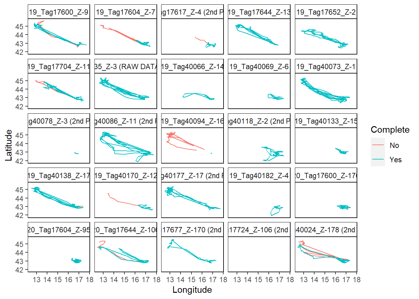
## If you want to map the trips from the next 25 animals tracked, use the IDs argument
mapTrips(trips = trips, IDs = 26:50, colony = colony_nest)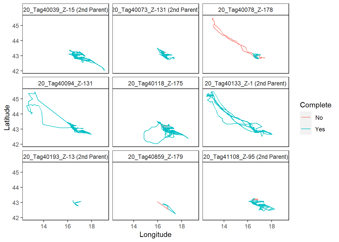
29.15.7 Plot the individual trips for each tracked animal after applying tripSplit()
If, after reviewing the simplified plots of individual trips for each tracked animal using the mapTrip() function you are not satisfied, then you should explore the relative data further.
One way of exploring the trips outputted for individually tracked animals would be to rapidly review summary plots for each trip, showing start, journey, and end points, where the point locations are also joined together with a line. Consider the code in the chapter Tracking data: Plotting tracks and reviewing tabular data
29.16 track2kba: What trip data to use (complete or incomplete trips)
Keeping points associated with complete trips only is the approach considered in the track2KBA online tutorial. But you may want to explore which trips you are keeping or not.
There are no definitive rules about what counts as a track good enough, or too bad, for an analysis. Users will need to consider the quality of the data obtained in relation to the species that was tracked and the key question they are exploring.
Users may wish to consider if too many individual trips have been removed. i.e. if you tracked 30 birds and you estimated to have approximately 3 trips recorded per bird, then you would have a total of 90 trips. But it’s likely that on some trips, that not the entire trip was recorded (for multiple reasons). Therefore, you might expect to rather have about 83 trips recorded across all birds because for 7 trips data might not have indicated birds returned to the colony. If you had a very high proportion of trips that did not return to the colony, then it’s likely that you have defined the parameters incorrectly for tripSplit() and you should reconsider better ecologically based estimates for these parameters. There is of course the chance that there are other issues (i.e. poor quality data obtained given device functionality) with your data which would warrant more detailed exploration.
## ~~~~~~~~~~~~~~~~~~~~~~~~~~~~~~~~~~~~~~~~~~~~~~~~~~~~~~~~~~~~~~~~~~~~~~~~~~~~~
## Keep points associated with individual trips ----
## Filter the data to only keep the points associated with individual trips that
## were recognised as complete trips.
## ~~~~~~~~~~~~~~~~~~~~~~~~~~~~~~~~~~~~~~~~~~~~~~~~~~~~~~~~~~~~~~~~~~~~~~~~~~~~~

## Let's first check how many trips we record as Yes vs. No before filtering
head(trips,2)
## x y dttm dataset_id
## 1200 42.811528 16.885531 2019-05-24 00:49:09 populated-upon-upload-STDB
## 2159 42.812029 16.886907 2019-05-24 01:09:03 populated-upon-upload-STDB
## scientific_name common_name site_name colony_name lat_colony
## 1200 Puffinus yelkouan Yelkouan Shearwater Lastovo SPA Z 42.774893
## 2159 Puffinus yelkouan Yelkouan Shearwater Lastovo SPA Z 42.774893
## lon_colony device ID track_id
## 1200 16.875649 GPS 19_Tag17600_Z-9 19_Tag17600_Z-9
## 2159 16.875649 GPS 19_Tag17600_Z-9 19_Tag17600_Z-9
## original_track_id age sex breed_stage
## 1200 populated-upon-upload-STDB adult unknown chick-rearing
## 2159 populated-upon-upload-STDB adult unknown chick-rearing
## breed_status date_gmt time_gmt argos_quality equinox
## 1200 populated-upon-upload-STDB 2019-05-24 00:49:09 NA NA
## 2159 populated-upon-upload-STDB 2019-05-24 01:09:03 NA NA
## Filter optional Latitude Longitude DateTime tripID
## 1200 TRUE TRUE 42.811528 16.885531 2019-05-24 00:49:09 19_Tag17600_Z-9_01
## 2159 TRUE TRUE 42.812029 16.886907 2019-05-24 01:09:03 19_Tag17600_Z-9_01
## X Y Returns StartsOut ColDist
## 1200 16.885531 42.811528 Yes Yes 4149.301440
## 2159 16.886907 42.812029 Yes Yes 4226.997952## summary of trips associated with Return or not
totalTripsAll <- data.frame(trips) %>% group_by(tripID, Returns) %>%
summarise(count = n()) %>%
data.frame(.)
## view summary result
table(totalTripsAll$Returns)##
## No Yes
## 1 19 325## NOW, Filter to only include trips that return
trips.return.yes <- subset(trips, trips$Returns == "Yes" )
totalTripsYes <- data.frame(trips.return.yes) %>% group_by(tripID, Returns) %>%
summarise(count = n()) %>%
data.frame(.)
## view summary result
table(totalTripsYes$Returns)##
## Yes
## 325## Filter for trips that do not reutrn
trips.return.no <- subset(trips, trips$Returns == "No" )
totalTripsNo <- data.frame(trips.return.no) %>% group_by(tripID, Returns) %>%
summarise(count = n()) %>%
data.frame(.)
## view summary result
table(totalTripsNo$Returns)##
## No
## 19##
## Yes
## 325##
## No
## 1929.16.1 track2KBA: Choice of complete trips only
If you want to explore further the trips that were not considered to have returned, then use the object above, trips.return.no, to investigate the individual trips further. E.g. through individual plotting.
For our example, we have 325 complete trips and 19 incomplete trips; a very small proportion of incomplete trips. We, therefore, deem our choice of input parameters as ecologically sensible for the tripSplit() function and use only the complete trips for further analyses.
29.17 track2KBA: Use only at-sea sections of trips
Key considerations related to identifying IBAs / KBAs: when identifying an IBA or KBA for seabirds using the track2KBA protocol, you effectively need information about the source population (typically the colony) and distribution data (tracking data). This means that not only can you identify a pelagic site from tracking data, but you can also consider an IBA/KBA for the colony itself and a possible at-sea buffer (seaward extension) around the colony.
Because you should typically consider identifying the seaward extension around the colony in addition to any potential pelagic / offshore sites supported by the tracking data, you can remove location points from the data within a suitable buffer distance (typically the inner buffer distance used in the tripSplit() function.
## remove locations near the vicinity of the colony - distance is in m (unlike innerBuff where distance was in km)
head(trips,2)
## x y dttm dataset_id
## 1200 42.811528 16.885531 2019-05-24 00:49:09 populated-upon-upload-STDB
## 2159 42.812029 16.886907 2019-05-24 01:09:03 populated-upon-upload-STDB
## scientific_name common_name site_name colony_name lat_colony
## 1200 Puffinus yelkouan Yelkouan Shearwater Lastovo SPA Z 42.774893
## 2159 Puffinus yelkouan Yelkouan Shearwater Lastovo SPA Z 42.774893
## lon_colony device ID track_id
## 1200 16.875649 GPS 19_Tag17600_Z-9 19_Tag17600_Z-9
## 2159 16.875649 GPS 19_Tag17600_Z-9 19_Tag17600_Z-9
## original_track_id age sex breed_stage
## 1200 populated-upon-upload-STDB adult unknown chick-rearing
## 2159 populated-upon-upload-STDB adult unknown chick-rearing
## breed_status date_gmt time_gmt argos_quality equinox
## 1200 populated-upon-upload-STDB 2019-05-24 00:49:09 NA NA
## 2159 populated-upon-upload-STDB 2019-05-24 01:09:03 NA NA
## Filter optional Latitude Longitude DateTime tripID
## 1200 TRUE TRUE 42.811528 16.885531 2019-05-24 00:49:09 19_Tag17600_Z-9_01
## 2159 TRUE TRUE 42.812029 16.886907 2019-05-24 01:09:03 19_Tag17600_Z-9_01
## X Y Returns StartsOut ColDist
## 1200 16.885531 42.811528 Yes Yes 4149.301440
## 2159 16.886907 42.812029 Yes Yes 4226.997952trips <- trips[trips$ColDist > inner.buff.distance*1000, ]
## Plot to review
## interactive plot - including colony location(s)
leaflet() %>% ## start leaflet plot
addProviderTiles(providers$Esri.WorldImagery, group = "World Imagery") %>%
## plot the points. Note: leaflet automatically finds lon / lat colonies
## Colour accordingly.
addCircleMarkers(data = data.frame(trips),
radius = 3,
fillColor = "cyan",
fillOpacity = 0.5, stroke = F) %>%
## plot the colony locations from birds
addCircleMarkers(data = data.frame(colony_nest),
radius = 5,
fillColor = "red",
fillOpacity = 0.5, stroke = F) Note: in the plot above, you may need to zoom into the colony of origin to ensure points have been removed accordingly.
29.18 track2KBA: Number of locations filter
It is worth considering the total number of location points contributing to each trip after splitting tracks from animals. Even if you are not splitting tracks into trips, using location data from animals where you have very few data points may bias your results.
Recommendation for the track2kba analytical approach is to use data with at least >5 location points
## create data frame and find IDs of trips with >5 locations; as required for track2KBA analysis
trips_to_keep <- data.frame(trips) %>%
  group_by(tripID) %>%
  summarise(triplocs = n()) %>%
  dplyr::filter(triplocs > 5)

## select the relevant tripIDs only and create new object
trips_df <- data.frame(trips) %>%
  dplyr::filter(tripID %in% trips_to_keep$tripID)

## Compare how many trips you removed
## Before
length(unique(trips$tripID))
## [1] 325## [1] 30529.19 track2KBA: tripSummary()
This will give us a guide to summary statistics about the tracking data from central place foraging animals.
## tripSummary() ----
sumTrips <- tripSummary(trips = trips_df, colony = colony_nest, nests = T)

## Check you only have complete trips here (if that is what you are aiming for)
table(sumTrips$complete)
##
## complete trip
## 305## filter for only complete trips if needed
#sumTrips <- sumTrips %>% dplyr::filter(complete= "complete trip")
## view output
head(sumTrips ,10)## # A tibble: 10 × 10
## # Groups: ID [2]
## ID tripID n_locs departure return duration
## <chr> <chr> <dbl> <dttm> <dttm> <dbl>
## 1 19_Tag17600_Z… 19_Ta… 46 2019-05-24 00:49:09 2019-05-30 06:27:14 150.
## 2 19_Tag17600_Z… 19_Ta… 9 2019-05-31 02:48:10 2019-05-31 12:28:30 9.67
## 3 19_Tag17600_Z… 19_Ta… 12 2019-06-02 03:07:31 2019-06-02 19:21:36 16.2
## 4 19_Tag17600_Z… 19_Ta… 73 2019-06-03 00:26:26 2019-06-08 16:19:49 136.
## 5 19_Tag17600_Z… 19_Ta… 9 2019-06-09 02:46:26 2019-06-09 11:47:30 9.02
## 6 19_Tag17604_Z… 19_Ta… 29 2019-05-05 20:10:16 2019-05-06 19:13:59 23.1
## 7 19_Tag17604_Z… 19_Ta… 17 2019-05-07 02:36:07 2019-05-07 15:32:41 12.9
## 8 19_Tag17604_Z… 19_Ta… 19 2019-05-08 02:58:44 2019-05-10 10:35:26 55.6
## 9 19_Tag17604_Z… 19_Ta… 8 2019-05-11 02:25:56 2019-05-12 03:44:00 25.3
## 10 19_Tag17604_Z… 19_Ta… 20 2019-05-13 04:36:26 2019-05-15 20:35:03 64.0
## # ℹ 4 more variables: total_dist <dbl>, max_dist <dbl>, direction <dbl>,
## # complete <chr>## [1] "19_Tag17600_Z-9" "19_Tag17604_Z-7"
## [3] "19_Tag17617_Z-4 (2nd Parent)" "19_Tag17644_Z-13"
## [5] "19_Tag17652_Z-2" "19_Tag17704_Z-11"
## [7] "19_Tag17735_Z-3 (RAW DATA MISSING)" "19_Tag40066_Z-14"
## [9] "19_Tag40069_Z-6" "19_Tag40073_Z-1"
## [11] "19_Tag40078_Z-3 (2nd Parent)" "19_Tag40086_Z-11 (2nd Parent)"
## [13] "19_Tag40094_Z-16" "19_Tag40118_Z-2 (2nd Parent)"
## [15] "19_Tag40133_Z-15" "19_Tag40138_Z-17"
## [17] "19_Tag40170_Z-12" "19_Tag40177_Z-17 (2nd Parent)"
## [19] "19_Tag40182_Z-4" "20_Tag17600_Z-170"
## [21] "20_Tag17604_Z-95" "20_Tag17644_Z-106"
## [23] "20_Tag17677_Z-170 (2nd Parent)" "20_Tag40024_Z-178 (2nd Parent)"
## [25] "20_Tag40039_Z-15 (2nd Parent)" "20_Tag40073_Z-131 (2nd Parent)"
## [27] "20_Tag40078_Z-178" "20_Tag40094_Z-131"
## [29] "20_Tag40118_Z-175" "20_Tag40133_Z-1 (2nd Parent)"
## [31] "20_Tag40193_Z-13 (2nd Parent)" "20_Tag40859_Z-179"
## [33] "20_Tag41108_Z-95 (2nd Parent)"## [1] 33## [1] 30529.19.1 Trip summary data review
NOTE: These metrics are just summaries of summary data. Additional methods (to be updated in future) may help you summarise your data in greater detail.
## Visual summary of data ----
## all data
all_tracks_sum <- sumTrips  %>% mutate(group = "all_tracks") %>%
  group_by(group) %>%
  summarise(n_trips = n(),
            avg_triptime_h = round(mean(duration),2),
            med_triptime_h = round(median(duration),2),
            min_triptime_h = round(min(duration),2),
            max_triptime_h = round(max(duration),2),
            avg_totdist_km = round(mean(total_dist),2),
            med_totdist_km = round(median(total_dist),2),
            min_totdist_km = round(min(total_dist),2),
            max_totdist_km = round(max(total_dist),2),
            avg_maxdist_km = round(mean(max_dist),2),
            med_maxdist_km = round(median(max_dist),2),
            min_maxdist_km = round(min(max_dist),2),
            max_maxdist_km = round(max(max_dist),2)) %>% data.frame()
## review all data summary
all_tracks_sum
## group n_trips avg_triptime_h med_triptime_h min_triptime_h
## 1 all_tracks 305 35.31 17.06 2.66
## max_triptime_h avg_totdist_km med_totdist_km min_totdist_km max_totdist_km
## 1 762.34 269.59 142.34 6.7 4609
## avg_maxdist_km med_maxdist_km min_maxdist_km max_maxdist_km
## 1 84.66 44.05 5.12 444.01## by individual
bird_sum <-
sumTrips %>%
group_by(ID) %>%
summarise(n_trips = n(),
avg_triptime_h = round(mean(duration),2),
med_triptime_h = round(median(duration),2),
min_triptime_h = round(min(duration),2),
max_triptime_h = round(max(duration),2),
avg_totdist_km = round(mean(total_dist),2),
med_totdist_km = round(median(total_dist),2),
min_totdist_km = round(min(total_dist),2),
max_totdist_km = round(max(total_dist),2),
avg_maxdist_km = round(mean(max_dist),2),
med_maxdist_km = round(median(max_dist),2),
min_maxdist_km = round(min(max_dist),2),
max_maxdist_km = round(max(max_dist),2)) %>% data.frame()
bird_sum## ID n_trips avg_triptime_h med_triptime_h
## 1 19_Tag17600_Z-9 5 64.09 16.23
## 2 19_Tag17604_Z-7 6 33.08 24.18
## 3 19_Tag17617_Z-4 (2nd Parent) 5 24.15 22.81
## 4 19_Tag17644_Z-13 2 216.26 216.26
## 5 19_Tag17652_Z-2 11 36.41 19.62
## 6 19_Tag17704_Z-11 7 64.81 19.07
## 7 19_Tag17735_Z-3 (RAW DATA MISSING) 13 45.94 16.59
## 8 19_Tag40066_Z-14 11 24.79 15.53
## 9 19_Tag40069_Z-6 14 24.44 16.66
## 10 19_Tag40073_Z-1 16 27.33 16.83
## 11 19_Tag40078_Z-3 (2nd Parent) 1 23.16 23.16
## 12 19_Tag40086_Z-11 (2nd Parent) 4 210.50 31.33
## 13 19_Tag40094_Z-16 1 23.70 23.70
## 14 19_Tag40118_Z-2 (2nd Parent) 12 23.33 17.13
## 15 19_Tag40133_Z-15 7 22.07 12.62
## 16 19_Tag40138_Z-17 4 152.82 110.77
## 17 19_Tag40170_Z-12 11 17.45 16.00
## 18 19_Tag40177_Z-17 (2nd Parent) 9 49.41 18.52
## 19 19_Tag40182_Z-4 14 22.48 18.25
## 20 20_Tag17600_Z-170 12 14.38 14.96
## 21 20_Tag17604_Z-95 16 24.43 17.30
## 22 20_Tag17644_Z-106 6 52.92 17.27
## 23 20_Tag17677_Z-170 (2nd Parent) 3 70.22 46.93
## 24 20_Tag40024_Z-178 (2nd Parent) 13 25.42 17.63
## 25 20_Tag40039_Z-15 (2nd Parent) 13 31.86 17.68
## 26 20_Tag40073_Z-131 (2nd Parent) 17 22.69 17.01
## 27 20_Tag40078_Z-178 4 17.00 17.70
## 28 20_Tag40094_Z-131 13 39.26 23.90
## 29 20_Tag40118_Z-175 23 23.59 15.36
## 30 20_Tag40133_Z-1 (2nd Parent) 13 33.49 18.40
## 31 20_Tag40193_Z-13 (2nd Parent) 3 38.64 14.24
## 32 20_Tag40859_Z-179 1 9.55 9.55
## 33 20_Tag41108_Z-95 (2nd Parent) 15 26.96 17.30
## min_triptime_h max_triptime_h avg_totdist_km med_totdist_km min_totdist_km
## 1 9.02 149.63 426.09 168.52 22.87
## 2 12.94 63.98 179.21 164.26 59.56
## 3 16.46 41.42 146.12 130.99 78.65
## 4 150.66 281.87 1685.70 1685.70 910.72
## 5 12.83 112.60 344.49 160.34 35.89
## 6 6.52 167.63 346.52 166.97 33.23
## 7 13.19 135.81 464.16 197.59 29.67
## 8 10.24 53.81 112.70 71.57 19.51
## 9 15.23 88.34 107.33 72.04 32.14
## 10 14.85 89.87 395.80 183.63 73.79
## 11 23.16 23.16 96.37 96.37 96.37
## 12 17.00 762.34 1248.77 153.49 79.10
## 13 23.70 23.70 23.11 23.11 23.11
## 14 5.00 64.57 179.18 149.39 6.70
## 15 2.66 85.67 122.93 70.61 17.08
## 16 37.21 352.52 990.90 752.76 26.88
## 17 15.00 23.00 111.00 104.56 52.84
## 18 14.85 186.36 411.98 71.66 29.86
## 19 12.05 66.83 114.22 87.89 26.74
## 20 8.38 15.83 122.94 121.95 60.93
## 21 8.31 84.67 132.59 134.70 56.13
## 22 14.24 138.14 391.11 136.04 44.98
## 23 25.97 137.75 553.84 148.70 83.45
## 24 12.42 108.91 226.86 152.27 92.17
## 25 16.09 137.00 261.92 183.71 107.62
## 26 14.62 63.02 180.11 145.14 108.81
## 27 13.97 18.64 135.35 133.90 111.50
## 28 8.39 115.15 289.18 169.64 46.63
## 29 12.50 138.11 220.88 168.03 83.02
## 30 15.07 92.05 397.71 202.89 61.68
## 31 14.09 87.59 113.34 32.54 26.45
## 32 9.55 9.55 101.23 101.23 101.23
## 33 15.35 68.34 197.54 154.83 113.21
## max_totdist_km avg_maxdist_km med_maxdist_km min_maxdist_km max_maxdist_km
## 1 1097.52 188.32 67.41 11.57 437.62
## 2 359.36 61.76 49.14 41.48 97.23
## 3 237.45 38.51 37.91 30.35 48.82
## 4 2460.68 365.05 365.05 318.96 411.13
## 5 1266.72 114.76 41.47 16.36 378.81
## 6 747.55 154.87 44.56 18.56 344.23
## 7 1364.57 166.73 35.96 17.13 433.62
## 8 483.83 44.05 24.28 6.44 222.64
## 9 422.01 32.82 29.26 13.33 101.08
## 10 1153.72 144.03 47.03 32.69 425.27
## 11 96.37 34.59 34.59 34.59 34.59
## 12 4609.00 152.27 77.17 34.36 420.39
## 13 23.11 12.89 12.89 12.89 12.89
## 14 509.72 53.36 43.12 5.12 154.98
## 15 311.77 42.16 29.61 9.36 109.13
## 16 2431.23 235.06 243.36 13.02 440.52
## 17 217.15 38.50 44.05 14.85 64.60
## 18 1713.08 115.73 20.64 12.97 428.56
## 19 306.02 33.40 30.36 13.65 107.76
## 20 175.58 44.77 40.47 25.77 71.27
## 21 299.72 43.12 39.48 25.27 75.57
## 22 1063.64 136.68 51.19 22.62 397.89
## 23 1429.38 168.92 46.91 37.19 422.66
## 24 1165.62 88.33 66.00 33.81 420.96
## 25 997.05 69.13 49.80 38.97 202.55
## 26 490.06 54.26 40.83 35.35 113.39
## 27 162.11 45.34 43.63 37.61 56.48
## 28 1237.56 97.34 72.24 32.38 440.35
## 29 987.00 64.10 49.95 29.89 171.85
## 30 1420.50 143.15 54.44 24.22 444.01
## 31 281.02 27.56 17.57 12.01 53.08
## 32 101.23 76.57 76.57 76.57 76.57
## 33 482.41 59.62 55.28 31.60 116.04## save the data as an excel sheet
#write.xlsx(bird_sum, file = "./Data/track2KBA_output/TrackingData_Summary.xlsx",
# sheetName = "Sheet1",
# col.names = TRUE, row.names = T, append = FALSE)
## histograms - foraging trip duration
p1 <- ggplot(sumTrips , aes(duration)) +
geom_histogram(colour = "darkgrey", fill = "cyan")+
theme(
axis.text=element_text(size=14, color="black"),
axis.title=element_text(size=16),
panel.background=element_rect(fill="white", colour="black")) +
ylab("n tracks") + xlab("Duration (hours)")
p1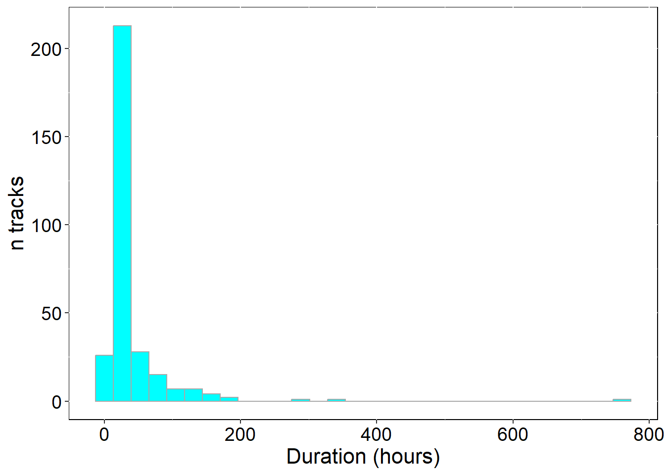
## total distance traveled from the colony
p2 <- ggplot(sumTrips , aes(total_dist)) +
  geom_histogram(colour = "darkgrey", fill = "cyan")+
  theme(
    axis.text=element_text(size=14, color="black"),
    axis.title=element_text(size=16),
    panel.background=element_rect(fill="white", colour="black")) +
  ylab("n tracks") + xlab("Total dist. travelled (km)")

p2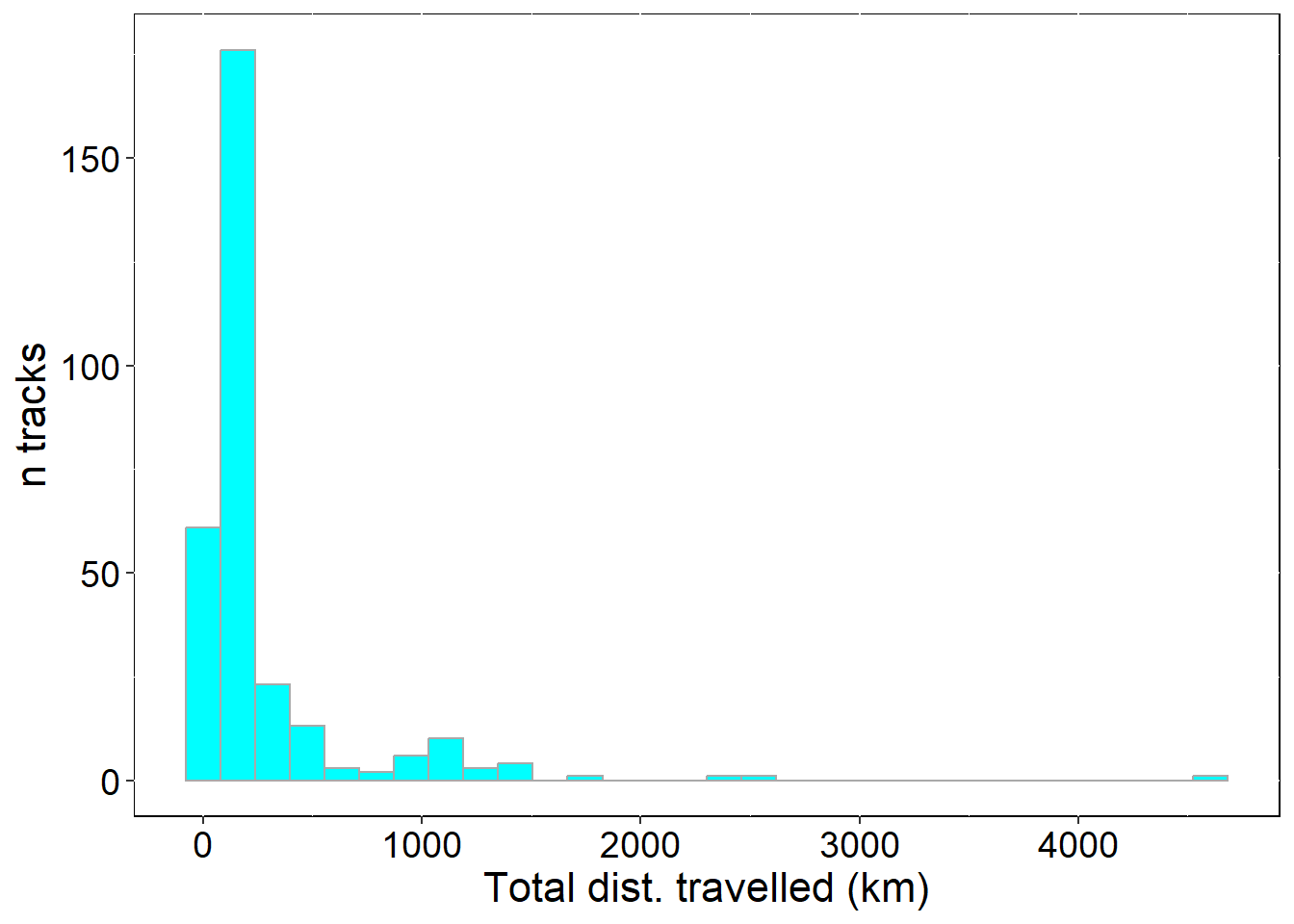
## maximum distance traveled from the colony
p3 <- ggplot(sumTrips , aes(max_dist)) +
  geom_histogram(colour = "darkgrey", fill = "cyan")+
  theme(
    axis.text=element_text(size=14, color="black"),
    axis.title=element_text(size=16),
    panel.background=element_rect(fill="white", colour="black")) +
  ylab("n tracks") + xlab("Max dist. from colony (km)")

p3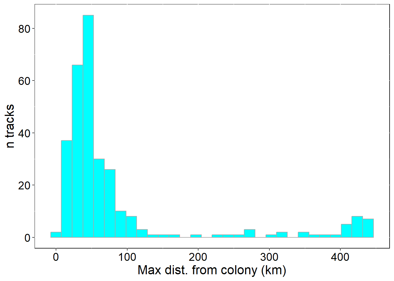
## save the plots
#ggsave(filename = paste("./Plots/HistSummary_Duration.png",sep=""),
#       p1,
#       dpi = 300, units = "mm", width = 180,height = 130)


#ggsave(filename = paste("./Plots/HistSummary_TotDist.png",sep=""),
#       p2,
#       dpi = 300, units = "mm", width = 180,height = 130)


#ggsave(filename = paste("./Plots/HistSummary_MaxDist.png",sep=""),
#       p3,
#       dpi = 300, units = "mm", width = 180,height = 130)
29.20 track2KBA: Sampling interval assessment
To implement track2KBA fully, you need data approximating an even sampling interval i.e. location points must be regularly spaced in time.
You must first determine how “gappy” the tracking data is (time intervals between location data)
This is an important step for almost all tracking data analyses.
If your data is not filtered / cleaned correctly, your ultimate results may be spurious.
#~~~~~~~~~~~~~~~~~~~~~~~~~~~~~~~~~~~~~~~~~~~~~~~~~~~~~~~~~~~~~~~~~~~~~~~~~~~~~~~
## Check sampling interval ----
#~~~~~~~~~~~~~~~~~~~~~~~~~~~~~~~~~~~~~~~~~~~~~~~~~~~~~~~~~~~~~~~~~~~~~~~~~~~~~~~

## data for summarising
head(data.frame(trips_df),2)
## x y dttm dataset_id
## 1200 42.811528 16.885531 2019-05-24 00:49:09 populated-upon-upload-STDB
## 2159 42.812029 16.886907 2019-05-24 01:09:03 populated-upon-upload-STDB
## scientific_name common_name site_name colony_name lat_colony
## 1200 Puffinus yelkouan Yelkouan Shearwater Lastovo SPA Z 42.774893
## 2159 Puffinus yelkouan Yelkouan Shearwater Lastovo SPA Z 42.774893
## lon_colony device ID track_id
## 1200 16.875649 GPS 19_Tag17600_Z-9 19_Tag17600_Z-9
## 2159 16.875649 GPS 19_Tag17600_Z-9 19_Tag17600_Z-9
## original_track_id age sex breed_stage
## 1200 populated-upon-upload-STDB adult unknown chick-rearing
## 2159 populated-upon-upload-STDB adult unknown chick-rearing
## breed_status date_gmt time_gmt argos_quality equinox
## 1200 populated-upon-upload-STDB 2019-05-24 00:49:09 NA NA
## 2159 populated-upon-upload-STDB 2019-05-24 01:09:03 NA NA
## Filter optional Latitude Longitude DateTime tripID
## 1200 TRUE TRUE 42.811528 16.885531 2019-05-24 00:49:09 19_Tag17600_Z-9_01
## 2159 TRUE TRUE 42.812029 16.886907 2019-05-24 01:09:03 19_Tag17600_Z-9_01
## X Y Returns StartsOut ColDist dataGroup.Longitude
## 1200 16.885531 42.811528 Yes Yes 4149.301440 16.885531
## 2159 16.886907 42.812029 Yes Yes 4226.997952 16.886907
## dataGroup.Latitude optional.1
## 1200 42.811528 TRUE
## 2159 42.812029 TRUE##
## Yes
## 9511## Determine difference between consecutive timestamps
## (NB: consecutive order of timestamps is critical here!)
## Doing this by tripID, not individual ID - change the group_by argument if needed
timeDiff <- trips_df %>%
data.frame() %>%
group_by(tripID) %>%
arrange(DateTime) %>%
mutate(delta_secs = as.numeric(difftime(DateTime, lag(DateTime, default = first(DateTime)), units = "secs"))) %>%
slice(2:n())
head(data.frame(timeDiff),2)## x y dttm dataset_id
## 1 42.812029 16.886907 2019-05-24 01:09:03 populated-upon-upload-STDB
## 2 42.811369 16.888280 2019-05-24 01:29:03 populated-upon-upload-STDB
## scientific_name common_name site_name colony_name lat_colony
## 1 Puffinus yelkouan Yelkouan Shearwater Lastovo SPA Z 42.774893
## 2 Puffinus yelkouan Yelkouan Shearwater Lastovo SPA Z 42.774893
## lon_colony device ID track_id original_track_id
## 1 16.875649 GPS 19_Tag17600_Z-9 19_Tag17600_Z-9 populated-upon-upload-STDB
## 2 16.875649 GPS 19_Tag17600_Z-9 19_Tag17600_Z-9 populated-upon-upload-STDB
## age sex breed_stage breed_status date_gmt time_gmt
## 1 adult unknown chick-rearing populated-upon-upload-STDB 2019-05-24 01:09:03
## 2 adult unknown chick-rearing populated-upon-upload-STDB 2019-05-24 01:29:03
## argos_quality equinox Filter optional Latitude Longitude DateTime
## 1 NA NA TRUE TRUE 42.812029 16.886907 2019-05-24 01:09:03
## 2 NA NA TRUE TRUE 42.811369 16.888280 2019-05-24 01:29:03
## tripID X Y Returns StartsOut ColDist
## 1 19_Tag17600_Z-9_01 16.886907 42.812029 Yes Yes 4226.997952
## 2 19_Tag17600_Z-9_01 16.888280 42.811369 Yes Yes 4181.804570
## dataGroup.Longitude dataGroup.Latitude optional.1 delta_secs
## 1 16.886907 42.812029 TRUE 1194
## 2 16.888280 42.811369 TRUE 1200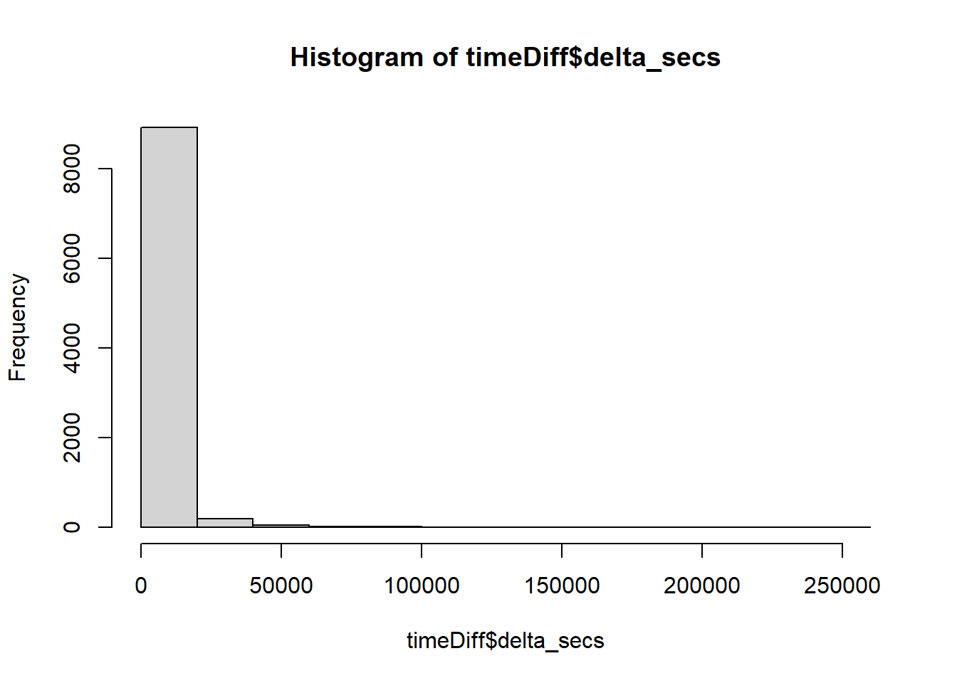
## plot histogram of timediff between all points
"This plot will take time depending on size of dataset!"## [1] "This plot will take time depending on size of dataset!"p4 <- ggplot(timeDiff , aes(delta_secs)) +
geom_histogram(colour = "darkgrey", fill = "cyan", binwidth = 200)+
theme(
axis.text=element_text(size=14, color="black"),
axis.title=element_text(size=16),
panel.background=element_rect(fill="white", colour="black")) +
ylab("n locations") + xlab("Time diff between locations (secs)")
p4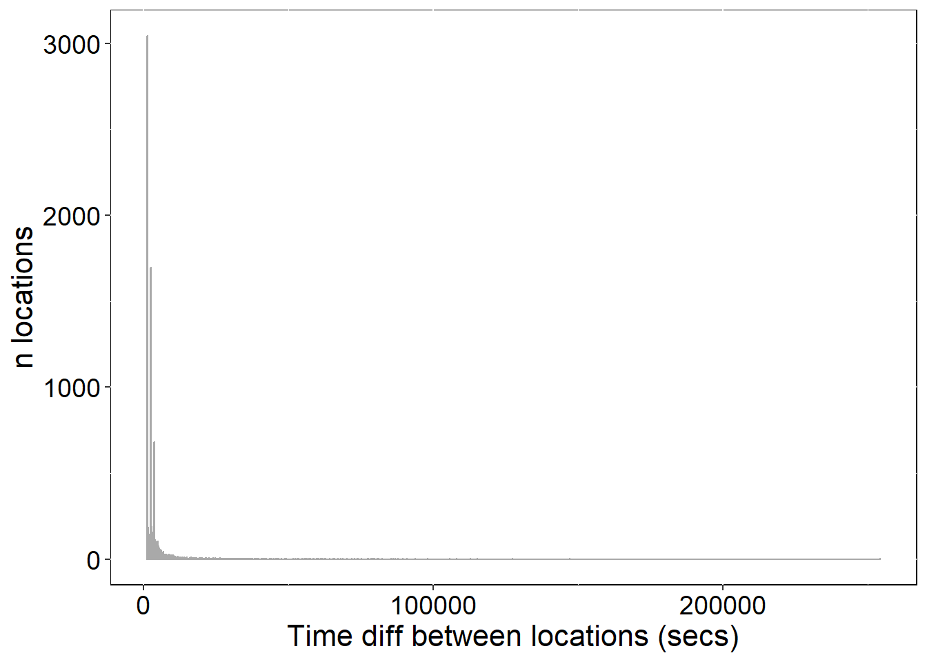
## Summarise results by tripID
SummaryTimeDiff <- timeDiff %>%
group_by(tripID) %>%
summarise(mean_timegap_secs = mean(delta_secs),
median_timegap_secs = median(delta_secs),
min_timegap_secs = min(delta_secs),
max_timegap_secs = max(delta_secs)) %>%
## time in days
mutate(max_timegap_days = max_timegap_secs / 86400) %>%
mutate(max_timegap_days = round(max_timegap_days,2)) %>%
data.frame()
## View results
SummaryTimeDiff## tripID mean_timegap_secs median_timegap_secs
## 1 19_Tag17600_Z-9_01 11970.777778 1205.0
## 2 19_Tag17600_Z-9_02 4352.500000 3998.5
## 3 19_Tag17600_Z-9_04 5313.181818 1484.0
## 4 19_Tag17600_Z-9_05 6794.486111 1209.0
## 5 19_Tag17600_Z-9_06 4058.000000 1729.0
## 6 19_Tag17604_Z-7_01 2965.107143 1733.0
## 7 19_Tag17604_Z-7_02 2912.125000 1318.0
## 8 19_Tag17604_Z-7_03 11122.333333 1791.0
## 9 19_Tag17604_Z-7_04 13012.000000 5800.0
## 10 19_Tag17604_Z-7_05 12121.947368 8574.0
## 11 19_Tag17604_Z-7_07 7920.500000 7955.0
## 12 19_Tag17617_Z-4 (2nd Parent)_01 2415.029412 2400.0
## 13 19_Tag17617_Z-4 (2nd Parent)_02 2547.454545 2403.0
## 14 19_Tag17617_Z-4 (2nd Parent)_03 3823.846154 2405.0
## 15 19_Tag17617_Z-4 (2nd Parent)_04 3291.722222 2504.0
## 16 19_Tag17617_Z-4 (2nd Parent)_05 3539.823529 2499.0
## 17 19_Tag17644_Z-13_01 7976.161765 1203.5
## 18 19_Tag17644_Z-13_02 6112.746988 1214.0
## 19 19_Tag17652_Z-2_01 1432.074074 1202.0
## 20 19_Tag17652_Z-2_02 2007.417910 1226.0
## 21 19_Tag17652_Z-2_03 3721.812500 2500.5
## 22 19_Tag17652_Z-2_05 2717.000000 2406.0
## 23 19_Tag17652_Z-2_06 2582.482759 2401.0
## 24 19_Tag17652_Z-2_07 2891.789474 2493.0
## 25 19_Tag17652_Z-2_08 4179.000000 3600.0
## 26 19_Tag17652_Z-2_09 3972.941176 3605.0
## 27 19_Tag17652_Z-2_10 4415.562500 3650.0
## 28 19_Tag17652_Z-2_11 4004.151899 3605.0
## 29 19_Tag17652_Z-2_12 3990.466667 3605.0
## 30 19_Tag17704_Z-11_01 2451.392857 1203.5
## 31 19_Tag17704_Z-11_02 2133.272727 1206.0
## 32 19_Tag17704_Z-11_03 4387.333333 1204.0
## 33 19_Tag17704_Z-11_05 12077.395833 3996.0
## 34 19_Tag17704_Z-11_06 4914.666667 2815.0
## 35 19_Tag17704_Z-11_07 10325.250000 2404.0
## 36 19_Tag17704_Z-11_08 12840.085106 7194.0
## 37 19_Tag17735_Z-3 (RAW DATA MISSING)_01 2923.529412 2442.0
## 38 19_Tag17735_Z-3 (RAW DATA MISSING)_02 3404.714286 2458.5
## 39 19_Tag17735_Z-3 (RAW DATA MISSING)_03 3934.333333 3676.0
## 40 19_Tag17735_Z-3 (RAW DATA MISSING)_04 4123.571429 3753.0
## 41 19_Tag17735_Z-3 (RAW DATA MISSING)_05 4593.000000 3738.0
## 42 19_Tag17735_Z-3 (RAW DATA MISSING)_06 5386.000000 3656.0
## 43 19_Tag17735_Z-3 (RAW DATA MISSING)_07 4984.802469 3768.0
## 44 19_Tag17735_Z-3 (RAW DATA MISSING)_08 3468.666667 2604.0
## 45 19_Tag17735_Z-3 (RAW DATA MISSING)_09 3653.384615 2562.0
## 46 19_Tag17735_Z-3 (RAW DATA MISSING)_10 3906.681818 2636.0
## 47 19_Tag17735_Z-3 (RAW DATA MISSING)_11 2677.000000 2429.0
## 48 19_Tag17735_Z-3 (RAW DATA MISSING)_12 5232.819672 3884.0
## 49 19_Tag17735_Z-3 (RAW DATA MISSING)_13 6697.438356 4153.0
## 50 19_Tag40066_Z-14_01 1531.490196 1205.0
## 51 19_Tag40066_Z-14_02 1716.656250 1214.0
## 52 19_Tag40066_Z-14_03 7168.166667 6397.0
## 53 19_Tag40066_Z-14_04 4608.500000 2838.5
## 54 19_Tag40066_Z-14_05 11184.400000 3886.0
## 55 19_Tag40066_Z-14_06 10592.615385 2476.0
## 56 19_Tag40066_Z-14_07 4969.100000 4964.0
## 57 19_Tag40066_Z-14_08 7770.000000 5633.0
## 58 19_Tag40066_Z-14_09 21523.777778 9549.0
## 59 19_Tag40066_Z-14_10 19439.285714 17101.0
## 60 19_Tag40066_Z-14_12 10079.500000 6852.0
## 61 19_Tag40069_Z-6_01 2968.600000 2452.0
## 62 19_Tag40069_Z-6_02 5782.236364 2689.0
## 63 19_Tag40069_Z-6_03 4578.769231 3821.0
## 64 19_Tag40069_Z-6_04 4654.846154 3609.5
## 65 19_Tag40069_Z-6_06 3654.333333 3602.0
## 66 19_Tag40069_Z-6_07 4098.071429 3600.5
## 67 19_Tag40069_Z-6_08 4646.615385 3622.0
## 68 19_Tag40069_Z-6_09 5494.000000 5016.0
## 69 19_Tag40069_Z-6_10 4677.923077 3931.0
## 70 19_Tag40069_Z-6_11 5144.727273 4430.0
## 71 19_Tag40069_Z-6_12 5017.454545 3779.0
## 72 19_Tag40069_Z-6_13 5047.896552 3612.0
## 73 19_Tag40069_Z-6_14 5311.916667 3870.5
## 74 19_Tag40069_Z-6_15 9678.000000 5653.5
## 75 19_Tag40073_Z-1_01 1451.047619 1201.0
## 76 19_Tag40073_Z-1_02 1511.108108 1204.0
## 77 19_Tag40073_Z-1_03 1505.897436 1208.0
## 78 19_Tag40073_Z-1_04 3562.866667 2697.0
## 79 19_Tag40073_Z-1_05 2896.500000 2449.0
## 80 19_Tag40073_Z-1_06 2694.739130 2402.0
## 81 19_Tag40073_Z-1_07 3116.105263 2592.0
## 82 19_Tag40073_Z-1_08 2518.400000 2400.0
## 83 19_Tag40073_Z-1_09 3352.277778 2408.5
## 84 19_Tag40073_Z-1_10 3315.794521 2405.0
## 85 19_Tag40073_Z-1_11 2535.458333 2401.0
## 86 19_Tag40073_Z-1_12 2922.894737 2401.0
## 87 19_Tag40073_Z-1_13 3423.294118 2663.0
## 88 19_Tag40073_Z-1_14 3321.125000 2415.5
## 89 19_Tag40073_Z-1_15 3332.421053 2848.0
## 90 19_Tag40073_Z-1_16 3635.179775 2418.0
## 91 19_Tag40078_Z-3 (2nd Parent)_01 1603.576923 1203.5
## 92 19_Tag40086_Z-11 (2nd Parent)_01 2464.285714 1221.0
## 93 19_Tag40086_Z-11 (2nd Parent)_02 4371.000000 1366.0
## 94 19_Tag40086_Z-11 (2nd Parent)_03 9979.694545 2400.0
## 95 19_Tag40086_Z-11 (2nd Parent)_06 13046.333333 6241.0
## 96 19_Tag40094_Z-16_01 17066.600000 1800.0
## 97 19_Tag40118_Z-2 (2nd Parent)_01 1200.000000 1200.0
## 98 19_Tag40118_Z-2 (2nd Parent)_02 2647.428571 1296.0
## 99 19_Tag40118_Z-2 (2nd Parent)_03 2923.326531 1252.0
## 100 19_Tag40118_Z-2 (2nd Parent)_04 3005.500000 1925.0
## 101 19_Tag40118_Z-2 (2nd Parent)_05 4280.500000 1715.5
## 102 19_Tag40118_Z-2 (2nd Parent)_06 3202.526316 1206.0
## 103 19_Tag40118_Z-2 (2nd Parent)_07 2554.318681 1205.0
## 104 19_Tag40118_Z-2 (2nd Parent)_08 3185.150000 1200.0
## 105 19_Tag40118_Z-2 (2nd Parent)_09 3469.722222 1205.5
## 106 19_Tag40118_Z-2 (2nd Parent)_10 3698.214286 1204.5
## 107 19_Tag40118_Z-2 (2nd Parent)_13 8984.571429 5934.0
## 108 19_Tag40118_Z-2 (2nd Parent)_14 6705.600000 3642.0
## 109 19_Tag40133_Z-15_01 1198.875000 1198.5
## 110 19_Tag40133_Z-15_02 6351.166667 4269.5
## 111 19_Tag40133_Z-15_03 9949.354839 2401.0
## 112 19_Tag40133_Z-15_06 10099.000000 8972.0
## 113 19_Tag40133_Z-15_08 3735.909091 2416.0
## 114 19_Tag40133_Z-15_10 7574.666667 5371.5
## 115 19_Tag40133_Z-15_11 12588.200000 2404.0
## 116 19_Tag40138_Z-17_01 5195.703704 1208.0
## 117 19_Tag40138_Z-17_03 7335.763006 2400.0
## 118 19_Tag40138_Z-17_04 9568.785714 6034.5
## 119 19_Tag40138_Z-17_05 6846.197917 3700.0
## 120 19_Tag40170_Z-12_01 1217.691176 1200.0
## 121 19_Tag40170_Z-12_02 1200.200000 1200.0
## 122 19_Tag40170_Z-12_04 2504.391304 2400.0
## 123 19_Tag40170_Z-12_05 2504.304348 2400.0
## 124 19_Tag40170_Z-12_06 2399.875000 2400.0
## 125 19_Tag40170_Z-12_07 2399.800000 2400.0
## 126 19_Tag40170_Z-12_08 2504.260870 2400.0
## 127 19_Tag40170_Z-12_09 2618.181818 2400.0
## 128 19_Tag40170_Z-12_10 2495.760000 2399.0
## 129 19_Tag40170_Z-12_11 3599.800000 3600.0
## 130 19_Tag40170_Z-12_12 3599.700000 3600.0
## 131 19_Tag40177_Z-17 (2nd Parent)_01 3154.833333 1272.0
## 132 19_Tag40177_Z-17 (2nd Parent)_02 2760.090909 1950.0
## 133 19_Tag40177_Z-17 (2nd Parent)_03 2969.222222 1467.5
## 134 19_Tag40177_Z-17 (2nd Parent)_04 2592.692708 1204.0
## 135 19_Tag40177_Z-17 (2nd Parent)_05 3397.650000 2262.5
## 136 19_Tag40177_Z-17 (2nd Parent)_06 3159.500000 2204.0
## 137 19_Tag40177_Z-17 (2nd Parent)_07 3174.857143 1751.0
## 138 19_Tag40177_Z-17 (2nd Parent)_08 4109.000000 2080.0
## 139 19_Tag40177_Z-17 (2nd Parent)_09 2879.343348 1203.0
## 140 19_Tag40182_Z-4_01 2400.151515 2400.0
## 141 19_Tag40182_Z-4_02 2550.882353 2400.0
## 142 19_Tag40182_Z-4_03 2446.074074 2402.0
## 143 19_Tag40182_Z-4_04 4275.285714 3602.0
## 144 19_Tag40182_Z-4_05 4666.931034 3628.0
## 145 19_Tag40182_Z-4_06 5595.395349 3604.0
## 146 19_Tag40182_Z-4_07 4688.250000 3914.5
## 147 19_Tag40182_Z-4_08 4797.571429 4011.0
## 148 19_Tag40182_Z-4_09 3911.058824 3602.0
## 149 19_Tag40182_Z-4_10 4851.529412 3763.0
## 150 19_Tag40182_Z-4_11 5446.333333 4110.5
## 151 19_Tag40182_Z-4_12 4526.636364 3671.0
## 152 19_Tag40182_Z-4_13 7577.750000 7529.5
## 153 19_Tag40182_Z-4_14 12042.600000 7651.0
## 154 20_Tag17600_Z-170_01 2860.368421 1451.0
## 155 20_Tag17600_Z-170_02 4255.916667 1935.5
## 156 20_Tag17600_Z-170_03 2403.260870 1712.0
## 157 20_Tag17600_Z-170_04 3562.000000 1203.0
## 158 20_Tag17600_Z-170_05 2943.666667 2034.5
## 159 20_Tag17600_Z-170_06 3717.466667 1279.0
## 160 20_Tag17600_Z-170_07 2188.480000 1239.0
## 161 20_Tag17600_Z-170_08 3349.687500 1332.5
## 162 20_Tag17600_Z-170_09 4134.230769 2405.0
## 163 20_Tag17600_Z-170_10 4420.909091 3076.0
## 164 20_Tag17600_Z-170_11 4307.142857 3284.0
## 165 20_Tag17600_Z-170_12 4904.545455 4029.0
## 166 20_Tag17604_Z-95_01 1800.346154 1202.5
## 167 20_Tag17604_Z-95_03 3328.352941 2347.0
## 168 20_Tag17604_Z-95_04 3708.733333 1668.0
## 169 20_Tag17604_Z-95_05 5773.000000 1248.0
## 170 20_Tag17604_Z-95_06 8958.200000 7644.0
## 171 20_Tag17604_Z-95_07 12119.545455 1201.0
## 172 20_Tag17604_Z-95_08 15574.777778 3668.0
## 173 20_Tag17604_Z-95_09 43546.000000 34250.0
## 174 20_Tag17604_Z-95_10 9722.000000 2404.0
## 175 20_Tag17604_Z-95_11 5484.000000 2513.0
## 176 20_Tag17604_Z-95_12 2992.700000 2265.0
## 177 20_Tag17604_Z-95_13 12209.000000 1202.0
## 178 20_Tag17604_Z-95_14 4358.933333 2602.0
## 179 20_Tag17604_Z-95_15 5589.300000 1850.5
## 180 20_Tag17604_Z-95_16 5403.666667 1831.5
## 181 20_Tag17604_Z-95_17 3894.650000 1202.5
## 182 20_Tag17644_Z-106_01 2847.611111 1202.5
## 183 20_Tag17644_Z-106_02 5180.229167 1200.5
## 184 20_Tag17644_Z-106_03 5105.500000 1203.0
## 185 20_Tag17644_Z-106_04 6102.000000 1201.0
## 186 20_Tag17644_Z-106_05 4719.329545 1201.0
## 187 20_Tag17644_Z-106_06 4203.600000 1586.0
## 188 20_Tag17677_Z-170 (2nd Parent)_01 18697.800000 4836.0
## 189 20_Tag17677_Z-170 (2nd Parent)_02 4427.776786 1201.0
## 190 20_Tag17677_Z-170 (2nd Parent)_03 8044.380952 1202.0
## 191 20_Tag40024_Z-178 (2nd Parent)_01 1446.333333 1207.5
## 192 20_Tag40024_Z-178 (2nd Parent)_02 1426.600000 1201.0
## 193 20_Tag40024_Z-178 (2nd Parent)_03 4919.636364 1253.0
## 194 20_Tag40024_Z-178 (2nd Parent)_04 2432.800000 1281.0
## 195 20_Tag40024_Z-178 (2nd Parent)_05 3229.882353 1257.0
## 196 20_Tag40024_Z-178 (2nd Parent)_06 4134.714286 1200.0
## 197 20_Tag40024_Z-178 (2nd Parent)_08 3322.711864 1202.0
## 198 20_Tag40024_Z-178 (2nd Parent)_09 5319.416667 1204.5
## 199 20_Tag40024_Z-178 (2nd Parent)_10 8273.428571 1335.0
## 200 20_Tag40024_Z-178 (2nd Parent)_11 5768.454545 1201.0
## 201 20_Tag40024_Z-178 (2nd Parent)_12 7764.111111 1204.5
## 202 20_Tag40024_Z-178 (2nd Parent)_13 6386.571429 3152.0
## 203 20_Tag40024_Z-178 (2nd Parent)_14 13321.000000 6989.0
## 204 20_Tag40039_Z-15 (2nd Parent)_01 1583.675000 1204.0
## 205 20_Tag40039_Z-15 (2nd Parent)_02 1353.893617 1205.0
## 206 20_Tag40039_Z-15 (2nd Parent)_03 2173.500000 1247.0
## 207 20_Tag40039_Z-15 (2nd Parent)_04 1863.647059 1203.0
## 208 20_Tag40039_Z-15 (2nd Parent)_05 1761.114286 1205.0
## 209 20_Tag40039_Z-15 (2nd Parent)_06 2187.000000 2398.5
## 210 20_Tag40039_Z-15 (2nd Parent)_07 2914.571429 2406.0
## 211 20_Tag40039_Z-15 (2nd Parent)_08 2896.400000 2585.5
## 212 20_Tag40039_Z-15 (2nd Parent)_09 3885.189189 2582.0
## 213 20_Tag40039_Z-15 (2nd Parent)_10 3275.295455 2682.0
## 214 20_Tag40039_Z-15 (2nd Parent)_11 2774.923077 1205.0
## 215 20_Tag40039_Z-15 (2nd Parent)_12 2722.280000 1598.0
## 216 20_Tag40039_Z-15 (2nd Parent)_13 4179.728814 1205.0
## 217 20_Tag40073_Z-131 (2nd Parent)_01 1549.000000 1205.0
## 218 20_Tag40073_Z-131 (2nd Parent)_02 1870.307692 1397.0
## 219 20_Tag40073_Z-131 (2nd Parent)_03 2320.203125 1360.0
## 220 20_Tag40073_Z-131 (2nd Parent)_04 2320.142857 1270.0
## 221 20_Tag40073_Z-131 (2nd Parent)_05 4014.266667 3249.0
## 222 20_Tag40073_Z-131 (2nd Parent)_06 4246.357143 3095.5
## 223 20_Tag40073_Z-131 (2nd Parent)_07 4080.214286 3493.0
## 224 20_Tag40073_Z-131 (2nd Parent)_08 3760.571429 2739.0
## 225 20_Tag40073_Z-131 (2nd Parent)_09 4896.583333 3799.0
## 226 20_Tag40073_Z-131 (2nd Parent)_10 5732.535714 3860.5
## 227 20_Tag40073_Z-131 (2nd Parent)_11 6122.600000 3597.5
## 228 20_Tag40073_Z-131 (2nd Parent)_12 3568.058824 2990.0
## 229 20_Tag40073_Z-131 (2nd Parent)_13 5928.111111 4525.0
## 230 20_Tag40073_Z-131 (2nd Parent)_14 4437.000000 3628.5
## 231 20_Tag40073_Z-131 (2nd Parent)_15 3178.150000 2928.0
## 232 20_Tag40073_Z-131 (2nd Parent)_16 3191.157895 2833.0
## 233 20_Tag40073_Z-131 (2nd Parent)_17 4931.782609 2841.5
## 234 20_Tag40078_Z-178_01 1967.281250 1251.5
## 235 20_Tag40078_Z-178_02 1733.965517 1203.0
## 236 20_Tag40078_Z-178_03 1973.823529 1226.0
## 237 20_Tag40078_Z-178_04 2223.103448 1446.0
## 238 20_Tag40094_Z-131_01 2098.292683 1203.0
## 239 20_Tag40094_Z-131_02 3929.810345 1776.5
## 240 20_Tag40094_Z-131_03 3776.000000 1315.0
## 241 20_Tag40094_Z-131_04 4934.845238 1201.0
## 242 20_Tag40094_Z-131_05 6620.333333 6260.5
## 243 20_Tag40094_Z-131_06 14867.000000 7024.0
## 244 20_Tag40094_Z-131_07 5619.684211 2214.5
## 245 20_Tag40094_Z-131_08 3537.500000 1201.5
## 246 20_Tag40094_Z-131_09 4503.000000 2181.0
## 247 20_Tag40094_Z-131_10 5998.727273 1203.0
## 248 20_Tag40094_Z-131_11 2864.814815 1203.0
## 249 20_Tag40094_Z-131_12 4906.058824 1206.0
## 250 20_Tag40094_Z-131_13 3781.609756 1206.0
## 251 20_Tag40118_Z-175_01 3284.235294 1444.0
## 252 20_Tag40118_Z-175_02 3347.882353 1373.0
## 253 20_Tag40118_Z-175_03 2647.058824 2154.0
## 254 20_Tag40118_Z-175_04 2453.000000 1526.5
## 255 20_Tag40118_Z-175_05 3578.153846 1819.0
## 256 20_Tag40118_Z-175_06 4685.100000 1472.5
## 257 20_Tag40118_Z-175_07 8926.500000 3240.0
## 258 20_Tag40118_Z-175_08 4537.090909 3099.0
## 259 20_Tag40118_Z-175_09 5353.900000 4584.5
## 260 20_Tag40118_Z-175_10 2169.125000 1886.0
## 261 20_Tag40118_Z-175_11 3335.600000 2502.0
## 262 20_Tag40118_Z-175_12 3950.857143 2994.0
## 263 20_Tag40118_Z-175_13 6943.875000 5236.0
## 264 20_Tag40118_Z-175_14 3613.352941 2577.0
## 265 20_Tag40118_Z-175_15 3274.588235 2594.0
## 266 20_Tag40118_Z-175_16 3907.764706 2737.0
## 267 20_Tag40118_Z-175_17 4117.270270 2841.0
## 268 20_Tag40118_Z-175_18 3732.133333 2726.0
## 269 20_Tag40118_Z-175_19 2628.380952 1933.0
## 270 20_Tag40118_Z-175_20 2463.913043 1928.0
## 271 20_Tag40118_Z-175_21 3166.751592 1370.0
## 272 20_Tag40118_Z-175_22 2834.000000 2420.0
## 273 20_Tag40118_Z-175_23 2227.144231 1240.0
## 274 20_Tag40133_Z-1 (2nd Parent)_01 1294.148936 1200.0
## 275 20_Tag40133_Z-1 (2nd Parent)_02 1796.536585 1208.5
## 276 20_Tag40133_Z-1 (2nd Parent)_03 1615.463415 1323.0
## 277 20_Tag40133_Z-1 (2nd Parent)_04 2821.000000 2452.5
## 278 20_Tag40133_Z-1 (2nd Parent)_05 2726.738636 2400.0
## 279 20_Tag40133_Z-1 (2nd Parent)_06 2890.500000 2403.5
## 280 20_Tag40133_Z-1 (2nd Parent)_07 3549.871795 2408.0
## 281 20_Tag40133_Z-1 (2nd Parent)_08 3401.250000 2629.0
## 282 20_Tag40133_Z-1 (2nd Parent)_09 2826.373494 2401.0
## 283 20_Tag40133_Z-1 (2nd Parent)_10 2914.521739 2411.0
## 284 20_Tag40133_Z-1 (2nd Parent)_11 2712.900000 2402.5
## 285 20_Tag40133_Z-1 (2nd Parent)_12 3270.722222 2453.0
## 286 20_Tag40133_Z-1 (2nd Parent)_13 2906.771930 2401.0
## 287 20_Tag40193_Z-13 (2nd Parent)_01 4228.333333 3603.5
## 288 20_Tag40193_Z-13 (2nd Parent)_02 4272.416667 3665.0
## 289 20_Tag40193_Z-13 (2nd Parent)_03 9009.114286 3988.0
## 290 20_Tag40859_Z-179_01 4299.750000 1433.5
## 291 20_Tag41108_Z-95 (2nd Parent)_01 1659.804598 1204.0
## 292 20_Tag41108_Z-95 (2nd Parent)_02 2425.967742 1797.0
## 293 20_Tag41108_Z-95 (2nd Parent)_03 1598.394737 1353.0
## 294 20_Tag41108_Z-95 (2nd Parent)_04 1946.812500 1209.5
## 295 20_Tag41108_Z-95 (2nd Parent)_05 2871.190476 1692.0
## 296 20_Tag41108_Z-95 (2nd Parent)_06 2403.000000 1845.0
## 297 20_Tag41108_Z-95 (2nd Parent)_07 3972.200000 3514.0
## 298 20_Tag41108_Z-95 (2nd Parent)_08 3095.421053 2406.0
## 299 20_Tag41108_Z-95 (2nd Parent)_09 3521.611111 3141.5
## 300 20_Tag41108_Z-95 (2nd Parent)_10 3089.979167 2412.0
## 301 20_Tag41108_Z-95 (2nd Parent)_11 3324.400000 2607.5
## 302 20_Tag41108_Z-95 (2nd Parent)_12 4521.692308 3242.0
## 303 20_Tag41108_Z-95 (2nd Parent)_13 8483.896552 3065.0
## 304 20_Tag41108_Z-95 (2nd Parent)_14 8180.620690 3984.0
## 305 20_Tag41108_Z-95 (2nd Parent)_15 5906.200000 2564.5
## min_timegap_secs max_timegap_secs max_timegap_days
## 1 1194 87842 1.02
## 2 1200 10478 0.12
## 3 1196 30663 0.35
## 4 1194 82303 0.95
## 5 1195 18016 0.21
## 6 1199 8904 0.10
## 7 1200 20248 0.23
## 8 1195 79438 0.92
## 9 2894 56196 0.65
## 10 2397 31853 0.37
## 11 2398 14803 0.17
## 12 1199 6296 0.07
## 13 2393 5411 0.06
## 14 2393 30424 0.35
## 15 2397 6840 0.08
## 16 2395 14346 0.17
## 17 1194 65797 0.76
## 18 1193 62651 0.73
## 19 1190 3565 0.04
## 20 1193 22457 0.26
## 21 2395 9069 0.10
## 22 2390 5148 0.06
## 23 2393 7779 0.09
## 24 2395 5266 0.06
## 25 2395 23922 0.28
## 26 3595 7605 0.09
## 27 3599 7739 0.09
## 28 3592 9326 0.11
## 29 3596 7767 0.09
## 30 1197 13949 0.16
## 31 1197 9175 0.11
## 32 1197 21956 0.25
## 33 2393 56912 0.66
## 34 2398 13942 0.16
## 35 2393 59759 0.69
## 36 3593 85464 0.99
## 37 2400 7980 0.09
## 38 2395 26298 0.30
## 39 3597 7398 0.09
## 40 3595 5366 0.06
## 41 3599 9523 0.11
## 42 3594 16483 0.19
## 43 2394 21593 0.25
## 44 2394 9511 0.11
## 45 2396 12628 0.15
## 46 2395 18735 0.22
## 47 2395 4184 0.05
## 48 3595 13224 0.15
## 49 3594 41815 0.48
## 50 1191 3805 0.04
## 51 1194 7593 0.09
## 52 2473 14965 0.17
## 53 2407 13036 0.15
## 54 2398 36048 0.42
## 55 2394 77485 0.90
## 56 2395 9761 0.11
## 57 2424 18115 0.21
## 58 3596 67044 0.78
## 59 4362 46261 0.54
## 60 3594 36814 0.43
## 61 2395 6049 0.07
## 62 2394 112755 1.31
## 63 3596 9973 0.12
## 64 3597 25196 0.29
## 65 3595 4383 0.05
## 66 3596 10125 0.12
## 67 3594 8728 0.10
## 68 3597 11352 0.13
## 69 3598 7592 0.09
## 70 3620 13722 0.16
## 71 3595 14060 0.16
## 72 3596 22571 0.26
## 73 3598 11304 0.13
## 74 4798 19939 0.23
## 75 1193 4155 0.05
## 76 1193 4349 0.05
## 77 1193 4087 0.05
## 78 2394 6339 0.07
## 79 2393 5211 0.06
## 80 2397 5955 0.07
## 81 2394 4900 0.06
## 82 2396 4895 0.06
## 83 2393 10957 0.13
## 84 2392 10227 0.12
## 85 2393 4803 0.06
## 86 2394 4988 0.06
## 87 2394 7729 0.09
## 88 2393 11983 0.14
## 89 2398 5935 0.07
## 90 2391 19152 0.22
## 91 1194 7066 0.08
## 92 1195 10813 0.13
## 93 1199 38827 0.45
## 94 1193 254116 2.94
## 95 3597 43321 0.50
## 96 1298 71850 0.83
## 97 1199 1201 0.01
## 98 1193 9920 0.11
## 99 1193 21739 0.25
## 100 1193 10909 0.13
## 101 1197 32856 0.38
## 102 1196 18122 0.21
## 103 1194 23220 0.27
## 104 1194 20039 0.23
## 105 1193 15215 0.18
## 106 1195 25392 0.29
## 107 1197 23431 0.27
## 108 1200 22212 0.26
## 109 1196 1203 0.01
## 110 1201 20233 0.23
## 111 2395 105548 1.22
## 112 2527 20578 0.24
## 113 2397 10119 0.12
## 114 2402 16608 0.19
## 115 2397 28484 0.33
## 116 1195 79645 0.92
## 117 1194 98046 1.13
## 118 2400 32094 0.37
## 119 3594 60399 0.70
## 120 1193 2399 0.03
## 121 1192 1208 0.01
## 122 2395 4800 0.06
## 123 2394 4798 0.06
## 124 2394 2406 0.03
## 125 2394 2406 0.03
## 126 2393 4801 0.06
## 127 2394 4794 0.06
## 128 2394 4806 0.06
## 129 3594 3606 0.04
## 130 3596 3606 0.04
## 131 1193 16141 0.19
## 132 1197 8320 0.10
## 133 1194 12636 0.15
## 134 1190 16720 0.19
## 135 1195 11702 0.14
## 136 1196 7861 0.09
## 137 1194 14754 0.17
## 138 1190 13989 0.16
## 139 1191 30191 0.35
## 140 2394 2406 0.03
## 141 2395 4805 0.06
## 142 2395 3231 0.04
## 143 3593 10417 0.12
## 144 3594 21370 0.25
## 145 3593 29188 0.34
## 146 3599 7794 0.09
## 147 3593 8512 0.10
## 148 3594 5862 0.07
## 149 3601 10864 0.13
## 150 3599 9842 0.11
## 151 3601 7583 0.09
## 152 3826 13324 0.15
## 153 3599 29484 0.34
## 154 1193 12898 0.15
## 155 1195 20638 0.24
## 156 1194 9878 0.11
## 157 1194 30361 0.35
## 158 1198 10394 0.12
## 159 1195 17638 0.20
## 160 1194 7008 0.08
## 161 1194 15725 0.18
## 162 1193 13829 0.16
## 163 2400 10417 0.12
## 164 2395 10509 0.12
## 165 2399 12334 0.14
## 166 1194 6048 0.07
## 167 1193 10908 0.13
## 168 1198 15200 0.18
## 169 1197 49038 0.57
## 170 1199 22573 0.26
## 171 1197 46503 0.54
## 172 1195 68526 0.79
## 173 2524 89374 1.03
## 174 2399 39623 0.46
## 175 1199 27215 0.31
## 176 1198 7941 0.09
## 177 1196 56009 0.65
## 178 1197 21335 0.25
## 179 1193 33992 0.39
## 180 1196 32957 0.38
## 181 1193 37006 0.43
## 182 1198 10277 0.12
## 183 1195 41429 0.48
## 184 1198 25529 0.30
## 185 1198 36684 0.42
## 186 1194 56382 0.65
## 187 1199 17128 0.20
## 188 1203 78426 0.91
## 189 1193 41269 0.48
## 190 1193 86879 1.01
## 191 1194 4452 0.05
## 192 1193 4764 0.06
## 193 1199 35581 0.41
## 194 1193 10651 0.12
## 195 1194 13284 0.15
## 196 1193 23370 0.27
## 197 1193 27494 0.32
## 198 1194 17387 0.20
## 199 1193 27407 0.32
## 200 1198 28963 0.34
## 201 1193 54504 0.63
## 202 1195 24038 0.28
## 203 1199 36344 0.42
## 204 1192 4656 0.05
## 205 1194 3260 0.04
## 206 1195 10297 0.12
## 207 1194 12515 0.14
## 208 1195 5621 0.07
## 209 1198 5222 0.06
## 210 2392 8788 0.10
## 211 2395 4836 0.06
## 212 2394 26374 0.31
## 213 2394 9629 0.11
## 214 1192 19298 0.22
## 215 1199 10282 0.12
## 216 1194 47305 0.55
## 217 1195 3987 0.05
## 218 1199 5077 0.06
## 219 1192 22631 0.26
## 220 1193 8049 0.09
## 221 1201 13653 0.16
## 222 2393 18533 0.21
## 223 2397 10592 0.12
## 224 2400 8110 0.09
## 225 2398 10416 0.12
## 226 2396 30407 0.35
## 227 2400 28809 0.33
## 228 2394 7369 0.09
## 229 2402 19297 0.22
## 230 2402 10958 0.13
## 231 2394 6758 0.08
## 232 2397 6730 0.08
## 233 2394 21533 0.25
## 234 1195 6367 0.07
## 235 1194 6052 0.07
## 236 1193 5623 0.07
## 237 1196 12306 0.14
## 238 1193 16365 0.19
## 239 1195 26174 0.30
## 240 1198 17025 0.20
## 241 1193 81078 0.94
## 242 1202 15554 0.18
## 243 1199 45084 0.52
## 244 1193 19638 0.23
## 245 1194 17039 0.20
## 246 1194 18962 0.22
## 247 1194 19855 0.23
## 248 1195 19938 0.23
## 249 1193 42092 0.49
## 250 1194 33496 0.39
## 251 1194 18242 0.21
## 252 1193 11891 0.14
## 253 1197 4862 0.06
## 254 1193 8143 0.09
## 255 1194 15736 0.18
## 256 1198 31345 0.36
## 257 1193 25498 0.30
## 258 1194 9950 0.12
## 259 1194 17821 0.21
## 260 1197 4563 0.05
## 261 2393 6745 0.08
## 262 2394 7451 0.09
## 263 2398 12932 0.15
## 264 2394 9371 0.11
## 265 2398 5349 0.06
## 266 2399 10998 0.13
## 267 2394 22303 0.26
## 268 2406 11733 0.14
## 269 1195 8603 0.10
## 270 1193 6207 0.07
## 271 1193 37412 0.43
## 272 1194 6132 0.07
## 273 1191 10499 0.12
## 274 1194 2823 0.03
## 275 1193 23979 0.28
## 276 1195 2711 0.03
## 277 2395 5069 0.06
## 278 2393 9235 0.11
## 279 2394 8836 0.10
## 280 2393 26398 0.31
## 281 2396 10132 0.12
## 282 2394 12276 0.14
## 283 2394 5590 0.06
## 284 2394 5675 0.07
## 285 2390 10634 0.12
## 286 2394 25644 0.30
## 287 3595 7203 0.08
## 288 3595 7237 0.08
## 289 3596 115169 1.33
## 290 1195 10918 0.13
## 291 1194 25145 0.29
## 292 1198 10174 0.12
## 293 1194 3904 0.05
## 294 1194 7784 0.09
## 295 1198 9840 0.11
## 296 1198 6821 0.08
## 297 2395 9900 0.11
## 298 2394 5883 0.07
## 299 2398 5697 0.07
## 300 2394 9518 0.11
## 301 2393 8756 0.10
## 302 2398 12709 0.15
## 303 2394 34433 0.40
## 304 2395 31484 0.36
## 305 2395 29146 0.34## tripID mean_timegap_secs median_timegap_secs min_timegap_secs
## 1 19_Tag17600_Z-9_01 11970.777778 1205.0 1194
## 2 19_Tag17600_Z-9_02 4352.500000 3998.5 1200
## 3 19_Tag17600_Z-9_04 5313.181818 1484.0 1196
## 4 19_Tag17600_Z-9_05 6794.486111 1209.0 1194
## 5 19_Tag17600_Z-9_06 4058.000000 1729.0 1195
## 6 19_Tag17604_Z-7_01 2965.107143 1733.0 1199
## max_timegap_secs max_timegap_days
## 1 87842 1.02
## 2 10478 0.12
## 3 30663 0.35
## 4 82303 0.95
## 5 18016 0.21
## 6 8904 0.1029.20.1 Sampling interval review
Consider whether the sampling interval of your tracking data is appropriate for formally running the track2KBA functions. Remember, the time differences between each of your location points should be equal (or close enough to equal) across all location points and individuals tracked. If the time difference between location points is not equal, the outputs you generate from track2KBA will not be valid because the underlying kernel density analysis implemented within the track2KBA functions will be invalid (because you need points evenly spaced in time for this analysis to be valid).
Therefore, review the summary of your recorded sampling interval data:
#~~~~~~~~~~~~~~~~~~~~~~~~~~~~~~~~~~~~~~~~~~~~~~~~~~~~~~~~~~~~~~~~~~~~~~~~~~~~~~~
## Review sampling interval ----
#~~~~~~~~~~~~~~~~~~~~~~~~~~~~~~~~~~~~~~~~~~~~~~~~~~~~~~~~~~~~~~~~~~~~~~~~~~~~~~~
## Average sampling interval of all data
## median of median time gaps in minutes
median(SummaryTimeDiff$median_timegap_secs)/60## [1] 40.03333333## Sort data by maximum time gap first - then view.
## Consider if you have any outlier trips with massively different time gaps.
SummaryTimeDiff %>% arrange(-max_timegap_secs) %>% head(10)## tripID mean_timegap_secs median_timegap_secs
## 1 19_Tag40086_Z-11 (2nd Parent)_03 9979.694545 2400
## 2 20_Tag40193_Z-13 (2nd Parent)_03 9009.114286 3988
## 3 19_Tag40069_Z-6_02 5782.236364 2689
## 4 19_Tag40133_Z-15_03 9949.354839 2401
## 5 19_Tag40138_Z-17_03 7335.763006 2400
## 6 20_Tag17604_Z-95_09 43546.000000 34250
## 7 19_Tag17600_Z-9_01 11970.777778 1205
## 8 20_Tag17677_Z-170 (2nd Parent)_03 8044.380952 1202
## 9 19_Tag17704_Z-11_08 12840.085106 7194
## 10 19_Tag17600_Z-9_05 6794.486111 1209
## min_timegap_secs max_timegap_secs max_timegap_days
## 1 1193 254116 2.94
## 2 3596 115169 1.33
## 3 2394 112755 1.31
## 4 2395 105548 1.22
## 5 1194 98046 1.13
## 6 2524 89374 1.03
## 7 1194 87842 1.02
## 8 1193 86879 1.01
## 9 3593 85464 0.99
## 10 1194 82303 0.95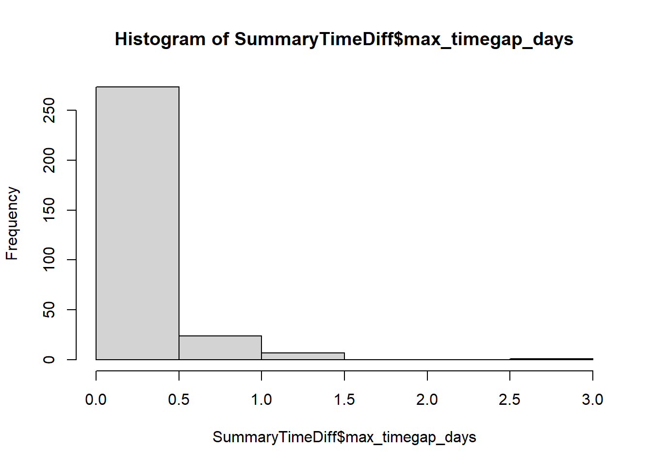
If you have trips where the maximum time gap in seconds (max_timegap_secs) is
extremely different to the median of median time gaps in minutes, then it’s likely you need to consider why this is the case for those trips.
- Did you specify tripSplit parameters incorrectly?
- Does the data require further cleaning in some other way?
- What else to consider
NOTE: you should be aware of what the original pre-programmed sampling interval was. How do your results compare to this interval?
29.21 track2KBA: Interpolating data for analysis
If you have gaps between time stamps in your tracking data, you need to fill these gaps for the purpose of the track2KBA protocol. It’s likely you will need to do this for many other tracking data analyses.
Broadly speaking, there are two key ways to fill the gaps in your tracking data, a process known as interpolation.
These two ways include:
Simpler linear interpolation
More advanced interpolation options that try account for where the animal could have moved (e.g. CRAWL)
Typically, for flying seabirds, where gaps in tracking data while birds at sea are less likely because birds do not typically dive underwater for durations as long as non-flying seabirds, linear interpolation should serve as a suitable starting point.
More advanced interpolation methods may be required for diving seabirds, or other diving marine predators.
See the appendix which offers an introduction to other available interpolation methods
29.21.1 Interpolating data: using only at-sea locations
REMINDER: Removing trip start and end points near the colony for the interpolation (as completed above), especially if using more advanced methods like CRAWL, can support filtering only points at sea when you estimate birds should be moving, as opposed to trying to deal with sections of trips when the bird is actually stationary on land.
Other methods do support interpolation of data when animals are on land. These are not yet detailed in the toolkit.
29.21.2 Interpolating data: choice of sampling interval
Reminder: The average sampling interval of all data (i.e. the median of median time gaps in minutes) was 40.0333333333 minutes.
Set your interpolation interval accordingly. You can use these results and knowledge of your programmed sampling interval.
Here we set the interpolation interval in minutes.
29.21.3 Interpolating data: linear interpolation implementation
Prior to implementing linear interpolation using available tools, we save a relevant version of the metadata because the interpolation functions often remove some of the additional metadata which are useful for later steps in the track2kba protocol.
##              x         y                dttm                 dataset_id
## 1200 42.811528 16.885531 2019-05-24 00:49:09 populated-upon-upload-STDB
## 2159 42.812029 16.886907 2019-05-24 01:09:03 populated-upon-upload-STDB
##        scientific_name         common_name   site_name colony_name lat_colony
## 1200 Puffinus yelkouan Yelkouan Shearwater Lastovo SPA           Z  42.774893
## 2159 Puffinus yelkouan Yelkouan Shearwater Lastovo SPA           Z  42.774893
##      lon_colony device              ID        track_id
## 1200  16.875649    GPS 19_Tag17600_Z-9 19_Tag17600_Z-9
## 2159  16.875649    GPS 19_Tag17600_Z-9 19_Tag17600_Z-9
##               original_track_id   age     sex   breed_stage
## 1200 populated-upon-upload-STDB adult unknown chick-rearing
## 2159 populated-upon-upload-STDB adult unknown chick-rearing
##                    breed_status   date_gmt time_gmt argos_quality equinox
## 1200 populated-upon-upload-STDB 2019-05-24 00:49:09            NA      NA
## 2159 populated-upon-upload-STDB 2019-05-24 01:09:03            NA      NA
##      Filter optional  Latitude Longitude            DateTime             tripID
## 1200   TRUE     TRUE 42.811528 16.885531 2019-05-24 00:49:09 19_Tag17600_Z-9_01
## 2159   TRUE     TRUE 42.812029 16.886907 2019-05-24 01:09:03 19_Tag17600_Z-9_01
##              X         Y Returns StartsOut     ColDist dataGroup.Longitude
## 1200 16.885531 42.811528     Yes       Yes 4149.301440           16.885531
## 2159 16.886907 42.812029     Yes       Yes 4226.997952           16.886907
##      dataGroup.Latitude optional.1
## 1200          42.811528       TRUE
## 2159          42.812029       TRUE
##
trips_meta <- trips_df %>%
dplyr::select(scientific_name,
common_name,
site_name,
colony_name,
lat_colony,
lon_colony,
bird_id = ID,
trip_id = tripID,
age,
sex,
breed_stage,
breed_status) %>%
group_by(trip_id) %>%
slice(1)
## Compare and ensure same number of trips across data
length(unique(trips_df$tripID))## [1] 305## [1] 305Now perform the interpolation on each unique trip in your data.
## start blank df
trips_interp_df <- data.frame()

for(i in 1:length(unique(trips_df$tripID))){

  temp <- trips_df %>% dplyr::filter(tripID == unique(trips_df$tripID)[i])

  ## Linear interpolation -----
  ## Apply linear interpolation step to speed filtered only data

  ## create ltraj object
  trip_lt <- as.ltraj(xy = bind_cols(x = temp$Longitude,
                                     y = temp$Latitude),
                      date = temp$DateTime,
                      id = temp$tripID)

  ## Linearly interpolate/re-sample tracks according to chose interval (specified in seconds)
  trip_interp <- redisltraj(trip_lt,
                            interp.interval * 60,
                            type="time")
  head(trip_interp)

  ## convert back into format for track2KBA - dataframe for now
  trip_interp <- ld(trip_interp) %>%
    dplyr::mutate(Longitude = x,
                  Latitude = y)

  ## bind back onto dataframe
  trips_interp_df <- rbind(trips_interp_df, trip_interp)

  ## remove temporary items before next loop iteration
  rm(temp,trip_lt)

  ## Print loop progress
  print(paste("Trip ", i, " of ", length(unique(trips_df$tripID)), " processed"))

}
## [1] "Trip 1 of 305 processed"
## [1] "Trip 2 of 305 processed"
## [1] "Trip 3 of 305 processed"
## [1] "Trip 4 of 305 processed"
## [1] "Trip 5 of 305 processed"
## [1] "Trip 6 of 305 processed"
## [1] "Trip 7 of 305 processed"
## [1] "Trip 8 of 305 processed"
## [1] "Trip 9 of 305 processed"
## [1] "Trip 10 of 305 processed"
## [1] "Trip 11 of 305 processed"
## [1] "Trip 12 of 305 processed"
## [1] "Trip 13 of 305 processed"
## [1] "Trip 14 of 305 processed"
## [1] "Trip 15 of 305 processed"
## [1] "Trip 16 of 305 processed"
## [1] "Trip 17 of 305 processed"
## [1] "Trip 18 of 305 processed"
## [1] "Trip 19 of 305 processed"
## [1] "Trip 20 of 305 processed"
## [1] "Trip 21 of 305 processed"
## [1] "Trip 22 of 305 processed"
## [1] "Trip 23 of 305 processed"
## [1] "Trip 24 of 305 processed"
## [1] "Trip 25 of 305 processed"
## [1] "Trip 26 of 305 processed"
## [1] "Trip 27 of 305 processed"
## [1] "Trip 28 of 305 processed"
## [1] "Trip 29 of 305 processed"
## [1] "Trip 30 of 305 processed"
## [1] "Trip 31 of 305 processed"
## [1] "Trip 32 of 305 processed"
## [1] "Trip 33 of 305 processed"
## [1] "Trip 34 of 305 processed"
## [1] "Trip 35 of 305 processed"
## [1] "Trip 36 of 305 processed"
## [1] "Trip 37 of 305 processed"
## [1] "Trip 38 of 305 processed"
## [1] "Trip 39 of 305 processed"
## [1] "Trip 40 of 305 processed"
## [1] "Trip 41 of 305 processed"
## [1] "Trip 42 of 305 processed"
## [1] "Trip 43 of 305 processed"
## [1] "Trip 44 of 305 processed"
## [1] "Trip 45 of 305 processed"
## [1] "Trip 46 of 305 processed"
## [1] "Trip 47 of 305 processed"
## [1] "Trip 48 of 305 processed"
## [1] "Trip 49 of 305 processed"
## [1] "Trip 50 of 305 processed"
## [1] "Trip 51 of 305 processed"
## [1] "Trip 52 of 305 processed"
## [1] "Trip 53 of 305 processed"
## [1] "Trip 54 of 305 processed"
## [1] "Trip 55 of 305 processed"
## [1] "Trip 56 of 305 processed"
## [1] "Trip 57 of 305 processed"
## [1] "Trip 58 of 305 processed"
## [1] "Trip 59 of 305 processed"
## [1] "Trip 60 of 305 processed"
## [1] "Trip 61 of 305 processed"
## [1] "Trip 62 of 305 processed"
## [1] "Trip 63 of 305 processed"
## [1] "Trip 64 of 305 processed"
## [1] "Trip 65 of 305 processed"
## [1] "Trip 66 of 305 processed"
## [1] "Trip 67 of 305 processed"
## [1] "Trip 68 of 305 processed"
## [1] "Trip 69 of 305 processed"
## [1] "Trip 70 of 305 processed"
## [1] "Trip 71 of 305 processed"
## [1] "Trip 72 of 305 processed"
## [1] "Trip 73 of 305 processed"
## [1] "Trip 74 of 305 processed"
## [1] "Trip 75 of 305 processed"
## [1] "Trip 76 of 305 processed"
## [1] "Trip 77 of 305 processed"
## [1] "Trip 78 of 305 processed"
## [1] "Trip 79 of 305 processed"
## [1] "Trip 80 of 305 processed"
## [1] "Trip 81 of 305 processed"
## [1] "Trip 82 of 305 processed"
## [1] "Trip 83 of 305 processed"
## [1] "Trip 84 of 305 processed"
## [1] "Trip 85 of 305 processed"
## [1] "Trip 86 of 305 processed"
## [1] "Trip 87 of 305 processed"
## [1] "Trip 88 of 305 processed"
## [1] "Trip 89 of 305 processed"
## [1] "Trip 90 of 305 processed"
## [1] "Trip 91 of 305 processed"
## [1] "Trip 92 of 305 processed"
## [1] "Trip 93 of 305 processed"
## [1] "Trip 94 of 305 processed"
## [1] "Trip 95 of 305 processed"
## [1] "Trip 96 of 305 processed"
## [1] "Trip 97 of 305 processed"
## [1] "Trip 98 of 305 processed"
## [1] "Trip 99 of 305 processed"
## [1] "Trip 100 of 305 processed"
## [1] "Trip 101 of 305 processed"
## [1] "Trip 102 of 305 processed"
## [1] "Trip 103 of 305 processed"
## [1] "Trip 104 of 305 processed"
## [1] "Trip 105 of 305 processed"
## [1] "Trip 106 of 305 processed"
## [1] "Trip 107 of 305 processed"
## [1] "Trip 108 of 305 processed"
## [1] "Trip 109 of 305 processed"
## [1] "Trip 110 of 305 processed"
## [1] "Trip 111 of 305 processed"
## [1] "Trip 112 of 305 processed"
## [1] "Trip 113 of 305 processed"
## [1] "Trip 114 of 305 processed"
## [1] "Trip 115 of 305 processed"
## [1] "Trip 116 of 305 processed"
## [1] "Trip 117 of 305 processed"
## [1] "Trip 118 of 305 processed"
## [1] "Trip 119 of 305 processed"
## [1] "Trip 120 of 305 processed"
## [1] "Trip 121 of 305 processed"
## [1] "Trip 122 of 305 processed"
## [1] "Trip 123 of 305 processed"
## [1] "Trip 124 of 305 processed"
## [1] "Trip 125 of 305 processed"
## [1] "Trip 126 of 305 processed"
## [1] "Trip 127 of 305 processed"
## [1] "Trip 128 of 305 processed"
## [1] "Trip 129 of 305 processed"
## [1] "Trip 130 of 305 processed"
## [1] "Trip 131 of 305 processed"
## [1] "Trip 132 of 305 processed"
## [1] "Trip 133 of 305 processed"
## [1] "Trip 134 of 305 processed"
## [1] "Trip 135 of 305 processed"
## [1] "Trip 136 of 305 processed"
## [1] "Trip 137 of 305 processed"
## [1] "Trip 138 of 305 processed"
## [1] "Trip 139 of 305 processed"
## [1] "Trip 140 of 305 processed"
## [1] "Trip 141 of 305 processed"
## [1] "Trip 142 of 305 processed"
## [1] "Trip 143 of 305 processed"
## [1] "Trip 144 of 305 processed"
## [1] "Trip 145 of 305 processed"
## [1] "Trip 146 of 305 processed"
## [1] "Trip 147 of 305 processed"
## [1] "Trip 148 of 305 processed"
## [1] "Trip 149 of 305 processed"
## [1] "Trip 150 of 305 processed"
## [1] "Trip 151 of 305 processed"
## [1] "Trip 152 of 305 processed"
## [1] "Trip 153 of 305 processed"
## [1] "Trip 154 of 305 processed"
## [1] "Trip 155 of 305 processed"
## [1] "Trip 156 of 305 processed"
## [1] "Trip 157 of 305 processed"
## [1] "Trip 158 of 305 processed"
## [1] "Trip 159 of 305 processed"
## [1] "Trip 160 of 305 processed"
## [1] "Trip 161 of 305 processed"
## [1] "Trip 162 of 305 processed"
## [1] "Trip 163 of 305 processed"
## [1] "Trip 164 of 305 processed"
## [1] "Trip 165 of 305 processed"
## [1] "Trip 166 of 305 processed"
## [1] "Trip 167 of 305 processed"
## [1] "Trip 168 of 305 processed"
## [1] "Trip 169 of 305 processed"
## [1] "Trip 170 of 305 processed"
## [1] "Trip 171 of 305 processed"
## [1] "Trip 172 of 305 processed"
## [1] "Trip 173 of 305 processed"
## [1] "Trip 174 of 305 processed"
## [1] "Trip 175 of 305 processed"
## [1] "Trip 176 of 305 processed"
## [1] "Trip 177 of 305 processed"
## [1] "Trip 178 of 305 processed"
## [1] "Trip 179 of 305 processed"
## [1] "Trip 180 of 305 processed"
## [1] "Trip 181 of 305 processed"
## [1] "Trip 182 of 305 processed"
## [1] "Trip 183 of 305 processed"
## [1] "Trip 184 of 305 processed"
## [1] "Trip 185 of 305 processed"
## [1] "Trip 186 of 305 processed"
## [1] "Trip 187 of 305 processed"
## [1] "Trip 188 of 305 processed"
## [1] "Trip 189 of 305 processed"
## [1] "Trip 190 of 305 processed"
## [1] "Trip 191 of 305 processed"
## [1] "Trip 192 of 305 processed"
## [1] "Trip 193 of 305 processed"
## [1] "Trip 194 of 305 processed"
## [1] "Trip 195 of 305 processed"
## [1] "Trip 196 of 305 processed"
## [1] "Trip 197 of 305 processed"
## [1] "Trip 198 of 305 processed"
## [1] "Trip 199 of 305 processed"
## [1] "Trip 200 of 305 processed"
## [1] "Trip 201 of 305 processed"
## [1] "Trip 202 of 305 processed"
## [1] "Trip 203 of 305 processed"
## [1] "Trip 204 of 305 processed"
## [1] "Trip 205 of 305 processed"
## [1] "Trip 206 of 305 processed"
## [1] "Trip 207 of 305 processed"
## [1] "Trip 208 of 305 processed"
## [1] "Trip 209 of 305 processed"
## [1] "Trip 210 of 305 processed"
## [1] "Trip 211 of 305 processed"
## [1] "Trip 212 of 305 processed"
## [1] "Trip 213 of 305 processed"
## [1] "Trip 214 of 305 processed"
## [1] "Trip 215 of 305 processed"
## [1] "Trip 216 of 305 processed"
## [1] "Trip 217 of 305 processed"
## [1] "Trip 218 of 305 processed"
## [1] "Trip 219 of 305 processed"
## [1] "Trip 220 of 305 processed"
## [1] "Trip 221 of 305 processed"
## [1] "Trip 222 of 305 processed"
## [1] "Trip 223 of 305 processed"
## [1] "Trip 224 of 305 processed"
## [1] "Trip 225 of 305 processed"
## [1] "Trip 226 of 305 processed"
## [1] "Trip 227 of 305 processed"
## [1] "Trip 228 of 305 processed"
## [1] "Trip 229 of 305 processed"
## [1] "Trip 230 of 305 processed"
## [1] "Trip 231 of 305 processed"
## [1] "Trip 232 of 305 processed"
## [1] "Trip 233 of 305 processed"
## [1] "Trip 234 of 305 processed"
## [1] "Trip 235 of 305 processed"
## [1] "Trip 236 of 305 processed"
## [1] "Trip 237 of 305 processed"
## [1] "Trip 238 of 305 processed"
## [1] "Trip 239 of 305 processed"
## [1] "Trip 240 of 305 processed"
## [1] "Trip 241 of 305 processed"
## [1] "Trip 242 of 305 processed"
## [1] "Trip 243 of 305 processed"
## [1] "Trip 244 of 305 processed"
## [1] "Trip 245 of 305 processed"
## [1] "Trip 246 of 305 processed"
## [1] "Trip 247 of 305 processed"
## [1] "Trip 248 of 305 processed"
## [1] "Trip 249 of 305 processed"
## [1] "Trip 250 of 305 processed"
## [1] "Trip 251 of 305 processed"
## [1] "Trip 252 of 305 processed"
## [1] "Trip 253 of 305 processed"
## [1] "Trip 254 of 305 processed"
## [1] "Trip 255 of 305 processed"
## [1] "Trip 256 of 305 processed"
## [1] "Trip 257 of 305 processed"
## [1] "Trip 258 of 305 processed"
## [1] "Trip 259 of 305 processed"
## [1] "Trip 260 of 305 processed"
## [1] "Trip 261 of 305 processed"
## [1] "Trip 262 of 305 processed"
## [1] "Trip 263 of 305 processed"
## [1] "Trip 264 of 305 processed"
## [1] "Trip 265 of 305 processed"
## [1] "Trip 266 of 305 processed"
## [1] "Trip 267 of 305 processed"
## [1] "Trip 268 of 305 processed"
## [1] "Trip 269 of 305 processed"
## [1] "Trip 270 of 305 processed"
## [1] "Trip 271 of 305 processed"
## [1] "Trip 272 of 305 processed"
## [1] "Trip 273 of 305 processed"
## [1] "Trip 274 of 305 processed"
## [1] "Trip 275 of 305 processed"
## [1] "Trip 276 of 305 processed"
## [1] "Trip 277 of 305 processed"
## [1] "Trip 278 of 305 processed"
## [1] "Trip 279 of 305 processed"
## [1] "Trip 280 of 305 processed"
## [1] "Trip 281 of 305 processed"
## [1] "Trip 282 of 305 processed"
## [1] "Trip 283 of 305 processed"
## [1] "Trip 284 of 305 processed"
## [1] "Trip 285 of 305 processed"
## [1] "Trip 286 of 305 processed"
## [1] "Trip 287 of 305 processed"
## [1] "Trip 288 of 305 processed"
## [1] "Trip 289 of 305 processed"
## [1] "Trip 290 of 305 processed"
## [1] "Trip 291 of 305 processed"
## [1] "Trip 292 of 305 processed"
## [1] "Trip 293 of 305 processed"
## [1] "Trip 294 of 305 processed"
## [1] "Trip 295 of 305 processed"
## [1] "Trip 296 of 305 processed"
## [1] "Trip 297 of 305 processed"
## [1] "Trip 298 of 305 processed"
## [1] "Trip 299 of 305 processed"
## [1] "Trip 300 of 305 processed"
## [1] "Trip 301 of 305 processed"
## [1] "Trip 302 of 305 processed"
## [1] "Trip 303 of 305 processed"
## [1] "Trip 304 of 305 processed"
## [1] "Trip 305 of 305 processed"## review it worked by checking total number of unique trips and comparing to original
length(unique(trips_df$tripID))## [1] 305## [1] 305## [1] 9511## [1] 21693Bind metadata back after interpolation. Because we lost the useful metadata after the interpolation step, bind this data back onto the outputted data following interpolation
## First create columns with same names
trips_interp_df <- trips_interp_df %>%
  rename(trip_id = id)

## Now bind the metadata back
trips_interp_df <- left_join(trips_interp_df,
                               trips_meta,
                               by = "trip_id")

## Review data
head(trips_interp_df,2)
## x y date dx dy
## 1 16.88553100 42.8115280 2019-05-24 00:49:09 0.002069365 0.0001677
## 2 16.88760037 42.8116957 2019-05-24 01:19:09 0.002553635 -0.0004107
## dist dt R2n abs.angle rel.angle
## 1 0.002076149030 1800 0.000000000e+00 0.08086264312 NA
## 2 0.002586450503 1800 4.310394793e-06 -0.15946401320 -0.2403266563
## trip_id burst pkey
## 1 19_Tag17600_Z-9_01 19_Tag17600_Z-9_01 19_Tag17600_Z-9_01.2019-05-24 00:49:09
## 2 19_Tag17600_Z-9_01 19_Tag17600_Z-9_01 19_Tag17600_Z-9_01.2019-05-24 01:19:09
## Longitude Latitude scientific_name common_name site_name
## 1 16.88553100 42.8115280 Puffinus yelkouan Yelkouan Shearwater Lastovo SPA
## 2 16.88760037 42.8116957 Puffinus yelkouan Yelkouan Shearwater Lastovo SPA
## colony_name lat_colony lon_colony bird_id age sex breed_stage
## 1 Z 42.774893 16.875649 19_Tag17600_Z-9 adult unknown chick-rearing
## 2 Z 42.774893 16.875649 19_Tag17600_Z-9 adult unknown chick-rearing
## breed_status
## 1 populated-upon-upload-STDB
## 2 populated-upon-upload-STDB29.22 Save data
Save relevant data for next steps of track2kba implementation
## create new folder within current working directory where you will save data
  ## first create the name of the species and the file path you need
  ## also use gsub to replace spaces within character strings (words) with a "-"
  species_name <- gsub(" ", "-", trips_interp_df$scientific_name[1])

  ## print the name for checking
  print(species_name)
## [1] "Puffinus-yelkouan" ## then create the new folder within current working directory
path_to_folder <- paste("./data-testing/tracking-data/",
species_name,"-track2kba-files",
sep="")
## print the file path name for checking
print(path_to_folder)## [1] "./data-testing/tracking-data/Puffinus-yelkouan-track2kba-files" ## Check if folder exists, and if it does not, then make a new folder
if (!file.exists(path_to_folder)) {
# If it does not exist, create a new folder
dir.create(path_to_folder)
print(paste("Created folder:", path_to_folder))
} else {
# do nothing, but let us know the folder exists already
print(paste("Folder already exists:", path_to_folder))
}## [1] "Folder already exists: ./data-testing/tracking-data/Puffinus-yelkouan-track2kba-files"## save updated file for next steps
write.csv(trips_interp_df, ## cleaned tracking data
file = paste0(path_to_folder,"/",species_name, "-input-tracks.csv"),
row.names = F)
write.csv(sumTrips, ## summary of overall trips data
file = paste0(path_to_folder,"/",species_name, "-input-summary.csv"),
row.names = F)